Information Technology | Artificial Intelligence » Glenn Shafer - Why Should Statisticians Be Interested in Artificial Intelligence

Source: http://www.doksinet Why Should Statisticians Be Interested in Artificial Intelligence? 1 Glenn Shafer 2 Statistics and artificial intelligence have much in common. Both disciplines are concerned with planning, with combining evidence, and with making decisions. Neither is an empirical science. Each aspires to be a general science of practical reasoning Yet the two disciplines have kept each other at arms length. Sometimes they resemble competing religions Each is quick to see the weaknesses in the others practice and the absurdities in the others dogmas. Each is slow to see that it can learn from the other. I believe that statistics and AI can and should learn from each other in spite of their differences. The real science of practical reasoning may lie in what is now the gap between them. I have discussed elsewhere how AI can learn from statistics (Shafer and Pearl, 1990). Here, since I am writing primarily for statisticians, I will emphasize how statistics can learn from

AI. I will make my explanations sufficiently elementary, however, that they can be understood by readers who are not familiar with standard probability ideas, terminology, and notation. I begin by pointing out how other disciplines have learned from AI. Then I list some specific areas in which collaboration between statistics and AI may be fruitful. After these generalities, I turn to a topic of particular interest to mewhat we can learn from AI about the meaning and limits of probability. I examine the probabilistic approach to combining evidence in expert systems, and I ask how this approach can be generalized to situations where we need to combine evidence but where the thorough-going use of numerical probabilities is impossible or inappropriate. I conclude that the most essential feature of probability in expert systemsthe feature we should try to generalizeis factorization, not conditional independence. I show how factorization generalizes from probability to numerous other

calculi for expert systems, and I discuss the implications of this for the philosophy of subjective probability judgment. This is a lot of territory. The following analytical table of contents may help keep it in perspective. Section 1. The Accomplishments of Artificial Intelligence Here I make the case that we, as statisticians, can learn from AI. Section 2. An Example of Probability Propagation This section is most of the paper. Using a simple example, I explain how probability 1This is the written version of a talk at the Fifth Annual Conference on Making Statistics Teaching More Effective in Schools of Business, held at the University of Kansas on June 1 and 2, 1990. 2Glenn Shafer is Ronald G. Harper Distinguished Professor, School of Business, University of Kansas, Lawrence, Kansas 66045. Research for this paper was partially supported by National Science Foundation grant IRI-8902444 The author would like to thank Paul Cohen, Pierre Ndilikilikesha, Ali Jenzarli, and Leen-Kiat

Soh for comments and assistance. Source: http://www.doksinet 2 judgments for many related events or variables can be constructed from local judgments (judgments involving only a few variables at a time) and how the computations to combine these judgments can be carried out locally. Section 3. Axioms for Local Computation In this section, I distill the essential features of the computations of the previous section into a set of axioms. These axioms apply not only to probability, but also to other calculi, numerical and non-numerical, that have been used to manage uncertainty in expert systems. Section 4. Artificial Intelligence and the Philosophy of Probability Is probability always the right way to manage uncertainty, even in AI? I argue that it is not. There is a continuum of problems, from those in which we can use probabilities to represent uncertainty and control reasoning to those where no explicit representation of uncertainty is useful. The axioms of the preceding section

extend farther into the middle ground between these extremes than probability itself. 1. The Accomplishments of Artificial Intelligence What has AI accomplished? Statisticians, among others, have been known to question whether it has accomplished much of anything. I hope to persuade you, however, that there are good reasons to be interested in AI in general and in the AI workshops in this conference in particular. The talented people who have worked in the field of AI during the past thirty years have accomplished a good deal. But there is a structural problem in recognizing their accomplishments as accomplishments of artificial intelligence. The problem is that once something artificial works, we no longer want to call it intelligent. Intelligence is supposed to be something mysterious, not something that we understand because we built it. The ideas and products that have come out of AI include time-sharing, electronic mail, the Macintosh personal computer interface, and expert

systems. These are all important, but are any of them intelligent? Of course not. In this respect, AI is similar to philosophy. It is hard to recognize the lasting achievements of philosophy as a discipline, because the successes of philosophy are absorbed by other disciplines or become new disciplines (such as physics, logic, and linguistics). To remain part of philosophy, a topic must be mystifying. About a decade ago, I heard Amos Tversky predict that AI would be remembered less for its own accomplishments than for its impact on more established disciplines. He contended that established disciplines often need the new ideas that can emerge from the unfettered thinking of a brash young discipline such as AI. They need these new ideas, and they are in a better position than AI itself to exploit them. They have the intellectual capital to do so Tverskys prediction has been borne out over the past decade. To see this, let us make a brief inventory of some disciplines AI has influenced:

computer science, psychology, philosophy, and mathematics. Computer Science. As I have already pointed out, many of the accomplishments of AI are now regarded simply as accomplishments of computer science. These include time-sharing, electronic mail, and many improvements in computer software and hardware. Source: http://www.doksinet 3 Psychology. The influence of AI on psychology is best summed up by the name “cognitive science.” This name covers a multitude of attitudes and accomplishments, and I am not well qualified to summarize them. Let me simply point out that cognitive science is much more willing to speculate about mechanism than the behaviorist approach to psychology that preceded it. The discipline of AI is only one of many disciplines that cognitive science has drawn on, but the AI ideathe idea of mind as computerhas been basic. For a balanced discussion of the historical roots of cognitive science, see Gardner (1985). Philosophy. In philosophy, as in psychology,

the last decade has seen a greater emphasis on mechanism and context. Philosophizing about concepts has drawn a little closer to the problems that would be involved in making a computer use these concepts. I cite as an example Jon Barwise and John Perrys work on situational semantics (Barwise and Perry 1983). This has its mathematical roots in logic, but it is driven by the desire to understand meaning in terms of mechanisms that are specific enough to be implemented. Mathematics. Few mathematicians would be sympathetic to the idea that AI has had much influence on their field. I submit, however, that something has had an influence As a discipline, mathematics is changing. The 1980s have seen a shift, symbolized by the David Report (David 1984), away from preoccupation with proof and towards greater emphasis on structure within mathematics and greater emphasis on the relation of mathematics to other disciplines. I challenge you to explain this shift, and I submit the hypothesis that

progress in symbolic formula manipulation and theorem-proving has been one of the principal causes. If computer programs can manipulate formulas and prove theorems (Bundy 1983, McAllester 1989), then it is no wonder that mathematicians now feel compelled to give a broader account of their expertise. Is it accidental that todays most thoughtful mathematicians talk about AI when they undertake to explain the real nature of their enterprise (see, e.g, Davis and Hersh 1986 and Kac, Rota, and Schwartz 1986)? I return now to our own field of statistics, hoping that I have persuaded you that being influenced by AI is not a sin. It would not put us in bad company to admit that some such influence exists. In fact, AI is influencing statistics, and this influence will grow. There are three basic areas of influence. First, intelligent software for data analysis is coming It will be useful, and it will cast new light on the craft of statistical modelling. Second, methods for handling data that

have been adopted with relatively little investigation in AI will come under our scrutiny and will contribute to our own toolbox of methods. Third, the struggle to use probability or probabilitylike ideas in expert systems will cast new light on the meaning and limits of probability Each of these three areas of influence is represented in this conference. Wayne Oldford, Paul Tukey, and Jacques LaFrance are talking about intelligent statistical software. Timothy Bell is talking about neural nets, one new method of data analysis from AI. Prakash Shenoy and Rajendra Srivastava are talking about belief functions in expert systems. The practical usefulness of intelligent statistical software is obvious. I want to comment also on its implications for understanding statistical modelling. Like other experts, we can easily become smug about our unique powers of judgment It is easy to denounce the failings of amateur users of statistics without spelling out in any generality how we would do it.

At the most fundamental level, the challenge of writing intelligent statistical software is the challenge of spelling out our expertise. If we know how to do it right, we should be able to explain how to do it right If the progress of expert systems in other areas is any guide, we will discover that this is both more complicated and more possible than we had thought. Source: http://www.doksinet 4 Statisticians have already begun to investigate methods of data analysis that have been proposed in AI. The work of White (1989) on neural nets is one example We have left some important methods relatively untouched, however. I cite as an example A G Ivakhnenkos group method of data handling and Roger Barrons learning networks, two closely related methods that have received more practical use than theoretical study (Farlow 1984). The third area I have pointed to, the implications of expert systems for the limits and meaning of probability, will be the topic of the rest of this paper. As I

have already explained, I will discuss how to generalize probability from the numerical theory with which we are familiar to more flexible tools for expert systems, and I will examine what we should learn about the philosophy of probability from this generalization. 2. An Example of Probability Propagation A number of statisticians and computer scientists, including Judea Pearl, David Spiegelhalter, Steffen Lauritzen, Prakash Shenoy, and myself, have explored the use of probability in expert systems (Pearl 1988, Shenoy and Shafer 1986, Lauritzen and Spiegelhalter 1988). Their work has led to new theoretical understanding and to improvements in actual expert systems. This work involves the manipulation of joint probability distributions in factored form. The factors are usually conditional probabilities involving only a few variables at a time. Such factors may be more practical to assess than joint probabilities involving many variables, and also more feasible to work with

computationally. The computational tasks include updating a joint distribution by conditioning on observations, marginalizing to find probabilities for values of individual variables, and finding configurations of values that are jointly most probable. These tasks can be carried out by processes of local computation and propagation that involve only a few variables at a time. We call each computation local because it involves only a few closely related variables, but a given local computation may incorporate evidence about distant variables that has been propagated through a sequence of other local computations involving successively less distant variables. In most of this work, the factorization is motivated by a causal model, but the probabilities are then given a subjective interpretation. The subjective interpretation is essential, because in most problems it is impossible to base probabilities for so many variables on observed frequenciesmost of the probabilities must be made up.

I will return to the issue of interpretation in Section 4. In this section, I will follow the usual subjective interpretation, not because I believe that it is really sensible to invent subjective distributions for large numbers of variables, but because the subjective interpretation is appropriate for the generalizations that I will consider later. Since this section is so long, it may be helpful to provide another analytical table of contents. Section 2.1 A Story with Pictures Here I tell a story about a burglar alarm. I draw a picture of the causal relationships among the variables in the story, I change it into a picture containing conditional probabilities, and I put these conditional probabilities together to form a factorization of a joint probability distribution. Section 2.2 Justifying the Factorization Here I derive the factorization of Section 2.1 from assumptions of conditional independence Source: http://www.doksinet 5 Section 2.3 Probabilities for Individual Variables

We saw in the first section that factorization allows us to construct many probabilities from a few probabilities. Here I show that it also allows the efficient computation of probabilities for individual variables. These benefits can be obtained from any factorization involving the same clusters of variables. The individual factors need not be probabilities. Section 2.4 Posterior Probabilities I want posterior probabilities about the burglar alarmprobability judgments that take all my information into account. The factorization we studied in the preceding sections is a factorization of the prior, not of the posterior. By adding an indicator function for each observed variable, we get a factorization of the posterior. This enables us to compute posterior probabilities for individual variables. Section 2.5 Join Trees Local computation works for the story of the burglar alarm because the clusters of variables involved in the factorization can be arranged in a join tree. In general, this

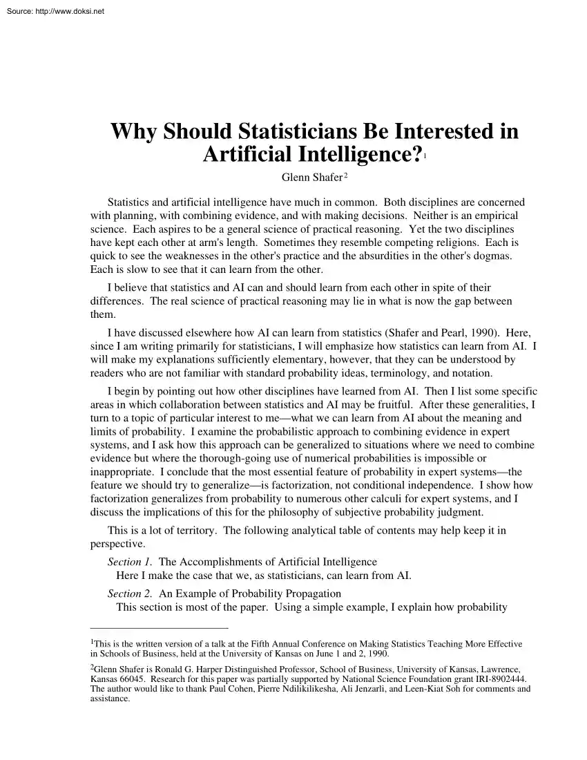
will not happen. To get a join tree, we must enlarge the clusters My purpose in this section is to make the simplicity of the ideas as clear as possible. I have not tried to be comprehensive. For a more thorough treatment, see Shafer and Shenoy (1988, 1990) E B Burglary Earthquake ER Figure 1. Earthquake reported on radio. EO EA Earthquake felt at office. Earthquake triggers alarm. The causal structure A of the story of the burglar Alarm goes off. alarm. AL PT Police try to call. PC I get police call. GW Gibbons is wacky. GP Gibbons played pranks in past week. Alarm loud enough for neighbors to hear. GH Gibbons hears the alarm. GC Call about alarm from Gibbons WH Watson hears the alarm. WC Confused call from Watson Source: http://www.doksinet 6 2.1 A Story with Pictures In this section, I tell a story about a burglar alarm, a story first told, in a simpler form, by Judea Pearl (1988, pp. 42-52) I draw a picture that displays the causal structure of this story

and then another picture that displays the conditional probabilities of the effects given their causes. I interpret this latter picture in terms of a factorization of my joint probability distribution for the variables in the story. Unlike the similar pictures drawn in path analysis (see, e.g, Duncan 1975), the pictures I draw here are not substantive hypotheses, to be tested by statistical data. Rather, they are guides to subjective judgement in a situation where there is little data relative to the number of variables being considered. We are using a presumed causal structure to guide the construction of subjective probabilities. The conditional probabilities are building blocks in that construction The Story. My neighbor Mr Gibbons calls me at my office at UCLA to tell me he has heard my burglar alarm go off. (No, I dont work at UCLA, but it is easiest to tell the story in the first person.) His call leaves me uncertain about whether my home has been burglarized The alarm might have

been set off instead by an earthquake. Or perhaps the alarm did not go off at all Perhaps the call is simply one of Gibbonss practical jokes. Another neighbor, Mr Watson, also calls, but I cannot understand him at all. I think he is drunk What other evidence do I have about whether there was an earthquake or a burglary? No one at my office noticed an earthquake, and when I switch the radio on for a few minutes, I do not hear any reports about earthquakes in the area. Moreover, I should have heard from the police if the burglar alarm went off. The police station is notified electronically when the alarm is triggered, and if the police were not too busy they would have called my office. Perhaps you found Figure 1 useful as you organized this story in your mind. It gives a rough picture of the storys causal structure. A burglary can cause the alarm to go off, hearing the alarm go off can cause Mr. Gibbons to call, etc Source: http://www.doksinet 7 E B Burglary Earthquake ER

Earthquake reported on radio. Figure 2. no EO EA Earthquake felt at office. Earthquake triggers alarm. no A The causal structure Alarm goes off. and the observations. PT AL Police try to call. PC I get police call. GW Gibbons is wacky. no GP Gibbons played pranks in past week. no Alarm loud enough for neighbors to hear. GH Gibbons hears the alarm. GC Call about alarm from Gibbons yes WH Watson hears the alarm. WC Confused call from Watson yes Source: http://www.doksinet 8 E B P(e) P(b) ER,EO,EA,E P( er,eo,ea | e ) Figure 3. EO ER EA The factorization A,EA,B of my prior distribution. P(a | ea,b) A PT,A AL,A P(pt | a) P(al | a) PT AL PC,PT GH,AL WH,AL P(pc | pt) P(gh | al) P(wh | al) PC GW P(gw) GH WH GP,GW GC,GW,GH WC,WH P(gp | gw) P(gc | gw,gh) P(wc | wh) GP GC WC Figure 1 shows only this causal structure. Figure 2 shows more; it also shows what I actually observed. Gibbons did not play any other pranks on me during the

preceding week (GP=no) Gibbons and Watson called (GC=yes, WC=yes), but the police did not (PC=no). I did not feel an earthquake at the office (EO=no), and I did not hear any report about an earthquake on the radio (ER=no). I will construct one subjective probability distribution based on the evidence represented by Figure 1, and another based on the evidence represented by Figure 2. Following the usual terminology of Bayesian probability theory, I will call the first my prior distribution, and second my posterior distribution. The posterior distribution is of greatest interest; it gives probabilities based on all my evidence. But we will study the prior distribution first, because it is much easier to work with. Only in Section 24 will we turn to the posterior distribution A Probability Picture. It is possible to interpret Figure 1 as a set of conditions on my subjective probabilities, but the interpretation is complicated. So I want to call your attention to a slightly different

picture, Figure 3, which conveys probabilistic information very directly. I have constructed Figure 3 from Figure 1 by interpolating a box between each child and its parents. In the box, I have put conditional probabilities for the child given the parents In one case (the case of E and its children, ER, EO, and EA), I have used a single box for several children. In other cases (such as the case of A and its children, PT and AL), I have used separate boxes for each child. I have also put unconditional probabilities in the circles that have no parents. Source: http://www.doksinet 9 The meaning of Figure 3 is simple: I construct my prior probability distribution for the fifteen variables in Figure 1 by multiplying together the functions (probabilities and conditional probabilities) in the boxes and circles: P(e,er,eo,ea,b,a,pt,pc,al,gh,wh,gw,gp,gc,wc) = P(e) . P(er,eo,ea|e) P(b) P(a|ea,b) P(pt|a) P(pc|pt) . P(al|a) P(gh|al) P(wh|al) P(gw) P(gp|gw) P(gc|gw,gh) P(wc|wh) (1) I

may not actually perform the multiplication numerically. But it defines my prior probability distribution in principle, and as we shall see, it can be exploited to find my prior probabilities for individual variables. I will call (1) a factorization of my prior probability distribution. This name can be misleading, for it suggests that the left-hand side was specified in some direct way and then factored. The opposite is true; we start with the factors and multiply them together, conceptually, to define the distribution. Once this is clearly understood, however, “factorization” is a useful word. Why should I define my prior probability distribution in this way? Why should I want or expect my prior probabilities to satisfy (1)? What use is the factorization? The best way to start answering these questions is to make the example numerical, by listing possible values of the variables and their numerical probabilities. This by itself will make the practical significance of the

factorization clearer, and it will give us a better footing for further abstract discussion. Frames. There are fifteen variables in my storyE, ER, EO, B, and so on The lower case letters in Figure 3e, er,eo, b, and so onrepresent possible values of these variables. What are these possible values? For simplicity, I have restricted most of the variables to two possible valuesyes or no. But in order to make the generality of the ideas clear, I have allowed two of the variables, PT and GW, to have three possible values. The police can try to call not at all, some, or a lot Mr Gibbonss level of wackiness this week can be low, medium, or high. This gives the sets of possible values shown in Figure 4. We can call these sets samples spaces or frames for the variables. Source: http://www.doksinet 10 yes no E Burglary Earthquake yes no ER Figure 4. Earthquake reported on radio. EO yes no B yes no Earthquake felt at office. EA yes no Earthquake triggers alarm. The frames. A

yes no Alarm goes off. not at all some a lot Police try to call. PT PC yes no I get police call. low GW medium high Gibbons is wacky. GP Gibbons played pranks in past week. yes no AL Alarm loud enough for neighbors to hear. yes no Gibbons hears the alarm. GH GC yes no yes no Call about alarm from Gibbons yes no Watson hears the alarm. WH WC yes no Confused call from Watson Probability Notation. The expressions in Figure 3 follow the usual notational conventions of probability theory: P(e) stands for “my prior probability that E=e,” P(a|ea,b) stands for “my prior probability that A=a, given that EA=ea and B=b,” P(er,eo,ea|e) stands for “my prior probability that ER=er and EO=eo and EA=ea, given that E=e,” and so on. Each of these expression stands not for a single number but rather for a whole set of numbersone number for each choice of values for the variables. In other words, the expressions stand for functions. This probability notation differs,

however, from the standard mathematical notation for functions. In mathematical notation, f(x) and g(x) are generally different functions, while f(x) and f(y) are the same function. Here, however, P(e) and P(b) are different functions The first gives my probabilities for E, while the second gives my probabilities for B. The Numbers. In Figure 5, I have replaced the expressions of Figure 3 with actual numbers The interpretation of these numbers should be self-evident. The numbers in the circle for E, for example, are P(E=yes) = .0001 and P(E=no) = 9999 The first number in the box below E is P(ER=yes & EO=yes & EA=yes | E=yes) = .01 And so on. Source: http://www.doksinet 11 E .0001 .9999 ER,EO,EA,E B - - - |yes - - - |no y,y,y .01 0 y,y,n .35 0 y,n,y .05 0 y,n,n .15 .01 n,y,y .03 0 P(er,eo,ea|e) n,y,n .20 .01 n,n,y .01 0 n,n,n .20 .98 ER EO .00001 .99999 EA A,EA,B - - |y,y - - |y,n - - |n,y - - |n,n y P(a|ea,b) 1 1 .7 . n 0 0 .3 . Figure 5. Actual numbers. A AL,A

PT,A - - |y - - |n n s l - - |y .6 .999998 P(pt|a) .2 .2 y n .000001 .000001 .6 P(al|a) .4 PT AL PC,PT y n - - |n - - |s P(pc|pt) 0 .4 1 .6 - - |l .8 .2 GH,AL .4 .3 .3 GP,GW y n -- |l .1 .9 -- |m -- |h .3 .8 .7 .2 GP WH,AL P(wh|al) - - |y - - |n P(gh|al) - - |y - - |n y n .5 .5 y n 0 1 GW PC - - |n 0 1 GH 0 1 WH GC,GW,GH -- |l,y -- |l,n -- |m,y -- |m,n -- |h,y -- |h,n y .8 .01 .7 .02 .6 .04 n .2 .99 .3 .98 .4 .96 GC .25 .75 WC,WH y n -- |y .2 .8 -- |n 0 1 WC The Probabilities of Configurations. Now that we have the numbers represented by the right-hand side of (1), we can compute the numbers represented by the left-hand side. This is important in principle, but in truth we are not directly interested in the numbers on the left-hand side. We are interested in them only in principle, because they determine the entire probability distribution. Just to illustrate the point, let us find the probability that the variables will come out the way shown in

Table 1. The first column of this table gives a value for each variable; in other words, it gives a configuration for the variables. The second column lists the probabilities that we must multiply together in order to obtain the probability of this configuration. Doing so, we find that the probability is approximately 10-8, or one in a hundred million. It is interesting that we can compute this number, but the number is not very meaningful by itself. When we have so many variables, most configurations will have a very small probability Without some standard of comparison, we have no way to give any direct significance to the probability of this configuration being one in a hundred million rather than one in a thousand or one in a billion. We are more interested in probabilities for values of individual variables. Figure 5 gives directly the probabilities for the values of E, B, and GW, but it does not give directly the probabilities for the other variables. It does not, for example,

tell us the probability that the alarm will go off. In principle, we can compute this from the probabilities of the configurations; Source: http://www.doksinet 12 we find the probabilities of all the configurations in which A=yes, and we add these probabilities up. As we will see in Section 23, however, there are much easier ways to find the probability that A=yes. For the sake of readers who are not familiar with probability theory, let me explain at this point two terms that I will use in this context: joint and marginal. A probability distribution for two or more variables is called a joint distribution. Thus the probability for a configuration is a joint probability. If we are working with a joint probability distribution for a certain set of variables, then the probability distribution for any subset of these variables, or for any individual variable, is called a marginal distribution. Thus the probability for an individual variable taking a particular value is a marginal

probability. Computing such probabilities is the topic of Section 2.3 Table 1. Computing the probability of a configuration. E=yes ER=yes EO=no EA=yes B=no A=yes PT=a lot PC=no AL=yes GH=yes WH=no GW=low GP=no GC=yes WC=no P(E=yes) 0.0001 P(ER=yes&EO=no&EA=yes|E=yes) 0.05 P(B=no) P(A=yes|EA=yes&B=no) P(PT=a lot|A=yes) P(PC=no|PT=a lot) P(AL=yes|A=yes) P(GH=yes|AL=yes) P(WH=no|AL=yes) P(GW=low) P(GP=no|GW=low) P(GC=yes|GW=low&GH=yes) P(WC=no|WH=no). 0.99999 1.0 0.2 0.2 0.6 0.5 0.75 0.4 0.9 0.8 1.0 Many Numbers from a Few. How many configurations of our fifteen variables are there? Since thirteen of the variables have two possible values and two of them have three possible values, there are 213 x 32 = 73,728 configurations altogether. One way to define my joint distribution for the fifteen variables would be to specify directly these 73,728 numbers, making sure that they add to one. Notice how much more practical and efficient it is to define it instead by means

of the factorization (1) and the 77 numbers in Figure 5. I could not directly make up sensible numerical probabilities for the 73,728 configurations Nor, for that matter, could I directly observe that many objective frequencies. But it may be practical to make up or observe the 77 probabilities on the right-hand side. It is also much more practical to store 77 rather than 73,728 numbers. We could make do with even fewer than 77 numbers. Since each column of numbers in the Figure 5 adds to one, we can leave out the last number in each column without any loss of information, and this will reduce the number of numbers we need to specify and store from 77 to 46. This reduction is unimportant, though, compared with the reduction from 73,728 to 77. Moreover, it is relatively illusory. When we specify the numbers, we do want to think about the Source: http://www.doksinet 13 last number in each column, to see that it makes sense. And it is convenient for computational purposes to store all

77 numbers. E B f(e) h(b) ER,EO,EA,E g(er,eo,ea,e) Figure 6. A general factorization. ER EO EA A,EA,B P(a|ea,b) i(a,ea,b) A PT,A P(pt|a) j(pt,a) PT PC,PT PC AL GH,AL P(gh|al) m(gh,al) P(pc|pt) k(pc,pt) GW GW P(gw) o(gw) GP,GW P(gp|gw) p(gp,gw) GP AL,A P(al|a) l(al,a) GH GC,GW,GH P(gc|gw,gh) q(gc,gw,gh) GC WH,AL P(wh|al) n(wh,al) WH WC,WH P(wc|wh) r(wc,wh) WC Other Factorizations. The fact that the factorization (1) allows us to specify and store the joint distribution efficiently does not depend on its right-hand side consisting of probabilities and conditional probabilities. We would do just as well with any factorization of the form P(e,er,eo,ea,b,a,pt,pc,al,gh,wh,gw,gp,gc,wc) = f(e) . g(er,eo,ea,e) h(b) i(a,ea,b) j(pt,a) k(pc,pt) . l(al,a) m(gh,al) n(wh,al) o(gw) p(gp,gw) q(gc,gw,gh) r(wc,wh), (2) no matter what the nature of the functions f, g, h, i, j, k, l, m, n, o, p, q, and r. Any such factorization would allow us to specify the

probabilities of the 73,728 configurations using only 77 numbers. Figure 6 displays the general factorization (2) in the same way that Figure 3 displays the special factorization (1). As I have just pointed out, Figure 6 is just as good as Figure 3 for specifying and storing a distribution. In Section 23, we will see that it is nearly as good for computing probabilities for individual variables. In Section 24, we will see that we have good reason for being interested in the greater generality. The special factorization for my prior distribution leads to the more general factorization for my posterior distribution. 2.2 Justifying the Factorization I have shown that the factorization displayed in Figure 3 is a convenient way to define my subjective probability distribution, but I have not explained its substantive meaning. What does it mean? How can I justify imposing it on my subjective probabilities? As I explain in this section, the factorization derives from my knowledge of the

causal structure sketched in Figure 1 and from the fact that my only evidence about the variables is my knowledge of this causal Source: http://www.doksinet 14 structure. (Remember that we are still talking about my prior probability distribution; I am pretending that I have not yet made the observations shown in Figure 2.) The explanation involves the probabilistic idea of independence. I am assuming that I know or can guess at the strength of the casual links in Figure 1. I know or can guess, that is to say, how often given values of the parents produce given values of the children. This means that my subjective probabilities will have the same structure as Figure 1. Links mean dependence with respect to my subjective probability distribution, and the absence of links means independence. Recall that independence of two variables, in subjective probability theory, means that information about one of the variables would not change my probabilities for the other. Formally, two

variables E and B are independent if P(b|e)=P(b), because P(b|e) is the probability I would have for B=b after I learned that E=e, and P(b) is the probability I would have for B=b before learning anything about E. These two variables should indeed be independent in our story, because there is no causal link from E to B or from B to E. Learning about the earthquake should not change my probabilities for the burglary, because there is no causal link I can use to justify the change. You may want to quibble here. Perhaps whether there is an earthquake would affect whether there is a burglary. Perhaps an earthquake would scare the burglars away, or send them scurrying home to look after their own broken windows. Perhaps, on the other side, an earthquake would bring out burglars looking for easy entrance into damaged houses. This illustrates that we can always think up new causal possibilities. We can question and reject any conditional independence relation. But at some point, we must

decide what is reasonable and what is too far-fetched to consider. I am telling this story, and I say that E and B are independent. Some independence relations are conditional. Consider, for example, the variables B, A, and AL in Figure 1. Here we say that AL and B are independent given A The fact that there is no direct link from B to AL means that B influences AL only through the intermediate variable A. (Aside from making the alarm go off, a burglary has no other influence on whether there is a sound from the alarm loud enough for the neighbors to hear.) This means that finding out whether the alarm went off will change my probabilities for there being a sound from it loud enough for the neighbors to hear, but after this, finding out whether there was a burglary will not make me change these probabilities further. Once I have learned that the alarm went off (A=yes), for example, and once I take this into account by changing my probability for AL from P(AL=yes) to P(AL=yes|A=yes),

further learning that there was a burglary (B=yes) will not make any difference; P(AL=yes|A=yes,B=yes) will be the same as P(AL=yes|A=yes). More generally, P(al|a,b)=P(al|a) for any choice of the values al, a, and b. To see how these independence relations lead to the factorization (1), we must first remember that any joint probability distribution can be factored into a succession of conditional probabilities, in many different ways. Without appealing to any independence relations, I can write P(e,er,eo,ea,b,a,pt,pc,al,gh,wh,gw,gp,gc,wc) = P(e) . P(er,eo,ea|e) P(b|e,er,eo,ea) P(a|e,er,eo,ea,b) . . P(each succeeding variable | all preceding variables) . (3) Source: http://www.doksinet 15 Here we have the probability for e, followed by the conditional probability for each succeeding variable given all the preceding ones, except that I have grouped er, eo, and ea together. There are thirteen factors altogether. Going from (3) to (1) is a matter of simplifying P(b|e,er,eo,ea)

to P(b), P(a|e,er,eo,ea,b) to P(a|ea,b), and so on. Each of these simplifications corresponds to an independence relation Consider the first factor, P(b|e,er,eo,ea). The variables E, ER, EO, and EA, which have to do with a possible earthquake, have no influence on B, whether there was a burglary. So B is unconditionally independent of E, ER, EO, and EA; knowing the values of E, ER, EO, and EA would not affect my probabilities for B. In symbols: P(b|e,er,eo,ea) = P(b) The next factor I need to simplify is P(a|e,er,eo,ea,b). Once I know whether or not an earthquake triggered the alarm (this is what the value of EA tells me) and whether there was a burglary, further earthquake information will not change further my probabilities about whether the alarm went off. So P(a|e,er,eo,ea,b) = P(a|ea,b); A is independent of E, ER, and EO given EA and B. I will leave it to the reader to simplify the remaining factors. In each case, the simplification is achieved by identifying my evidence with the

causal structure and then making a judgment of independence based on the lack of direct causal links. In each case, the judgment is that the variable whose probability is being considered is independent of the variables we leave out given the variables we leave in. One point deserves further discussion. In Figure 3, I used one box for the three children of E but separate boxes for the children of A and separate boxes for the children of GW. This choice, which is reflected in children of E entering (1) together while the children of A and GW enter separately, is based on my judgment that the children of E are dependent given E, while the children in the other cases are independent given their parents. This again is based on causal reasoning. In my version of the story, PT and AL are independent given A The mechanism by which the alarm alerts the police is physically independent of the mechanism by which it makes noise; hence if it goes off, whether it is loud enough for the neighbors to

hear is independent of whether the police try to call. On the other hand, if there is an earthquake at my home, whether it is strong enough to be felt at my office is not independent of whether it is important enough to be reported on the radio or strong enough to trigger my burglar alarm. Factorization or Independence? Since I have used independence relations to justify my factorization, you might feel that I should have started with independence rather than with factorization. Isnt it more basic? Most authors, including Pearl (1988) and Lauritzen and Spiegelhalter (1988) have emphasized independence rather than factorization. These authors do not use pictures such as Figure 3. Instead, they emphasize directed acyclic graphs, pictures like Figure 1, which they interpret directly as sets of independence relations. There are several reasons to emphasize factorization rather than independence. First, and most importantly, it is factorization rather than independence that generalizes most

fruitfully from probability to other approaches to handling uncertainty in expert systems. This is my message in Sections 3 and 4 of this paper. Second, even within the context of probability, an emphasis on independence obscures the essential simplicity of the local computations that we will study shortly. Local computation requires factorization, but it does not require all the independence relations implied by a directed acyclic graph. This is of practical importance when we undertake to compute posterior Source: http://www.doksinet 16 probabilities, for in this case we start only with a factorization. An insistence on working with a directed acyclic graph for the posterior will lead to conceptual complication and computational inefficiency. Third, the theory of independence is a detour from the problems of most importance. Only some of the independence relations suggested by the absence of links in Figure 1 were needed to justify the factorization. Do these imply the others?

What other subsets of all the independence relations suggested by the figure are sufficient to imply the others? These are interesting and sometimes difficult questions (see, e.g, Geiger 1990), but they have minimal relevance to computation and implementation 2.3 Probabilities for Individual Variables In Section 2.1, I pointed out that the factorizations of Figures 3 and 6 allow me to specify and store probabilities for many configurations using only a few numbers. In this section, we will study a second benefit of these factorizations. They allow me to compute the marginal probabilities for individual variables efficiently, using only local computations. I begin by demonstrating how to obtain marginals from Figure 3. The method is simple, and readers practiced in probability calculations will see immediately why it works. Then I will explain how to obtain marginals for the more general factorization of Figure 6. As we will see, there is slightly more work to do in this case, but the

generality of the case makes the simplicity of the method clear. We do not need the more subtle properties of probabilistic conditional independence. We need only the distributivity of multiplication over addition and a property of tree used by Figures 3 and 6it is a join tree. Marginals from the Special Factorization. Suppose we want my probabilities for A, whether the alarm went off. Figure 7 shows how to find them from the factorization of Figure 3 First we compute the marginal for EA. Then we use it to compute the marginal for A This is practical and efficient. It avoids working with all 73,728 configurations, which we would have to do if we had defined the joint directly, without a factorization. In the first step, we have two summations (one for EA=yes and one for EA=no), each involving only eight terms. In the second step, we again have two summations, each involving only four terms. We can compute the marginal for any variable we want in this way. We simply keep going down the

tree until we come to that variable. At each step, we compute the marginal for a particular variable from factors that involve only it and its parents. These factors are either given in the beginning or computed in the preceding steps. Source: http://www.doksinet 17 E B P(e) P(b) P(er,eo,ea|e) Figure 7. Computing marginals step-by-step down the ER EA EO Step 1: P(ea) = Σ [P(e)P(er,eo,ea|e)] P(a|ea,b) e,er,eo tree. A Step 2: Σ[ ] P(al|a) P(pt|a) P(ea)P(b)P(a|ea,b) P(a) = ea,b AL PT P(gh|al) P(pc|pt) GW PC P(wh|al) GH P(gw) P(gp|gw) WH P(gc|gw,gh) GP P(wc|wh) GC WC E .0001 .9999 ER,EO,EA,E Figure 8. ER EO .010055 .989945 B EA .00001 .99999 .00001 .99999 .010058 .989942 Marginal probabilities A,EA,B A for the individual variables. .00202 .99798 PT,A AL,A PT AL .99919 .000405 .000405 GH,AL PC,PT PC .000486 .999514 .001212 .998788 GW .4 .3 .3 GH WH,AL WH .000606 .999394 .000303 .999697 GP,GW GC,GW,GH WC,WH GP GC .37

.63 .02242 .97758 WC .0000606 .9999394 Source: http://www.doksinet 18 Figure 8 shows the numerical results, using the inputs of Figure 5. Each circle now contains the marginal probabilities for its variable. Why does this method work? Why are the formulas in Figure 7 correct? If you are practiced enough with probability, you may feel that the validity of the formulas and the method is too obvious to require much explanation. Were you to try to spell out an explanation, however, you would find it fairly complex. I will spell out an explanation, but I will do it in a roundabout way, in order to make clear the generality of the method. I will begin by redescribing the method in a leisurely way This will help us sort out what depends on the particular properties of the special factorization in Figure 3 from what will work for the general factorization in Figure 6. The Leisurely Redescription. My redescription involves pruning branches as I go down the tree of Figure 3. For reasons

that will become apparent only in Section 25, I prune very slowly At each step, I prune only circles or only boxes. On the first step, I prune only circles from Figure 3. I prune the circle E, the circle B, the circle ER, and the circle EO. When I prune a circle that contains a function (E and B contain functions, but ER and EO do not), I put that function in the neighboring box, where it multiplies the function already there. This gives Figure 9 On the next step, I prune the box ER,EO,EA,E from Figure 9. I sum the variables ER, EO, and E out of the function in the box, and I put the result, P(ea) in the neighboring circle. This gives Figure 10. Next I prune the circle EA, putting the factor it contains into the neighboring box. This gives Figure 11. Then I prune the box A,EA,B. I sum the variables EA and B out of the function in this box, and I put the result, P(a), in the neighboring circle. This gives Figure 12 Here are the rules I am following: Rule 1. I only prune twigs (A twig is

a circle or box that has only one neighbor; the circle EO is a twig in Figure 3, and the box A,EA,B is a twig in Figure 11.) Rule 2. When I prune a circle, I put its contents, if any, in the neighboring box, where it will be multiplied by whatever is already there. Rule 3. When I prune a box, I sum out from the function it contains any variables that are not in the neighboring circle, and then I put the result in that circle. In formulating Rules 2 and 3, I have used the fact that a twig in a tree has a unique neighbor. It is useful to have a name for this unique neighbor; I call it the twigs branch. I ask you to notice two properties of the process governed by these rules. First, in each figure, from Figure 9 to Figure 12, the functions in the boxes and the circles form a factorization for the joint probability distribution of the variables that remain in the picture. Second, the function I put into a circle is always the marginal probability distribution for the variable in that

circle. The second property is convenient, because it is the marginal probability distributions that we want. But as we will see shortly, the first property is more general It will hold when we prune the general factorization of Figure 6, while the second property will not. Moreover, the first property will hold when we prune twigs from below just as it holds when we prune twigs from above. This means that the first property is really all we need If we can prune twigs while Source: http://www.doksinet 19 retaining a factorization, and if we can prune twigs from below as well as from above, then we can obtain the marginal for a particular variable simply by pruning twigs from above and below until only that variable is left. You may have noticed that even with the special factorization of Figure 3, I am no longer pruning twigs if I keep moving down the tree after I have obtained Figure 12. The circle A is not a twig in Figure 12. Since I am working with the special factorization, I

can remove A nonetheless. I can put P(a) in both boxes below this circle Then I have two disconnected trees, and I can continue computing marginals, working down both trees. But this depends on the properties of the special factorization. When we work with the general factorization, we must rely on pruning twigs. ER,EO,EA,E P(e) P(er,eo,ea|e) EA EA P(ea) A,EA,B A,EA,B P(b) P(a|ea,b) P(b) P(a|ea,b) A A PT,A AL,A PT,A AL,A P(pt|a) P(al|a) P(pt|a) P(al|a) PT PT AL AL PC,PT GH,AL WH,AL PC,PT GH,AL WH,AL P(pc|pt) P(gh|al) P(wh|al) P(pc|pt) P(gh|al) P(wh|al) GW PC GP,GW WH GH P(gw) GC,GW,GH WC,WH P(gc|gw,gh) P(wc|wh) P(gp|gw) GP GC GW PC GP,GW GC,GW,GH WC,WH P(gc|gw,gh) P(wc|wh) P(gp|gw) GP WC Figure 9. WH GH P(gw) GC WC Figure 10. A,EA,B P(ea) P(b) P(a|ea,b) A A PT,A AL,A PT,A AL,A P(pt|a) P(al|a) P(pt|a) P(al|a) PT PC P(a) AL PT AL PC,PT GH,AL WH,AL PC,PT GH,AL WH,AL P(pc|pt) P(gh|al) P(wh|al) P(pc|pt)

P(gh|al) P(wh|al) GW P(gw) GP,GW P(gp|gw) GP GH WH GC,GW,GH WC,WH P(gc|gw,gh) P(wc|wh) GC WC PC GW P(gw) GP,GW P(gp|gw) GP GH WH GC,GW,GH WC,WH P(gc|gw,gh) P(wc|wh) GC WC Source: http://www.doksinet 20 Figure 11. Figure 12. Marginals from the General Factorization. Now I prune the general factorization of Figure 6. Figures 13 to 16 show what happens as I prune the circles and boxes above A Notice that I must invent some names for the functions I get when I sum out the variables. Going from Figure 13 to Figure 14 involves summing ER, EO, and E out of f(e).g(er,eo,ea,e); I arbitrarily call the result g*(ea). In symbols: g*(ea) = ∑ [f(e).g(er,eo,ea,e)] e,er,eo Similarly, i*(a) is the result of summing EA and B out of g(ea).h(b)i(a,ea,b): i*(a) = ∑ [g(ea).h(b)i(a,ea,b)] ea,b I want to convince you that Figures 13 to 16 have the same property as Figure 6. In each case, the functions in the picture constitute a factorization of the joint probability

distribution for the variables in the picture. ER,EO,EA,E f(e) g(er,eo,ea,e) EA EA g*(ea) A,EA,B A,EA,B P(a|ea,b) h(b) i(a,ea,b) P(a|ea,b) h(b) i(a,ea,b) A PT,A P(pt|a) j(pt,a) PT PC,PT PC GW GW P(gw) o(gw) GP,GW P(gp|gw) p(gp,gw) GP AL,A PT,A P(al|a) l(al,a) P(pt|a) j(pt,a) AL GH,AL P(gh|al) m(gh,al) P(pc|pt) k(pc,pt) A GH GC,GW,GH P(gc|gw,gh) q(gc,gw,gh) GC Figure 13. PT PC,PT WH,AL P(wh|al) n(wh,al) WH WC,WH P(wc|wh) r(wc,wh) WC PC AL GH,AL P(gh|al) m(gh,al) P(pc|pt) k(pc,pt) GW GW P(gw) o(gw) GP,GW P(gp|gw) p(gp,gw) GP AL,A P(al|a) l(al,a) GH GC,GW,GH P(gc|gw,gh) q(gc,gw,gh) GC WH,AL P(wh|al) n(wh,al) WH WC,WH P(wc|wh) r(wc,wh) WC Figure 14. Figure 13 obviously has this property, because it has the same functions as Figure 6. It is less obvious that Figure 14 has the property. It is here that we must use the distributivity of multiplication. In general, to obtain the joint distribution of a set of variables from the joint

distribution of a larger set of variables, we must sum out the variables that we want to omit. So if we omit ER, EO, and E from the joint distribution of all fifteen variables, the joint distribution of the twelve that remain is given by Source: http://www.doksinet 21 P(ea,b,a,pt,pc,al,gh,wh,gw,gp,gc,wc) = ∑ P(e,er,eo,ea,b,a,pt,pc,al,gh,wh,gw,gp,gc,wc) . e,er,eo When we substitute the factorization of Figure 6 in the right-hand side, this becomes P(ea,b,a,pt,pc,al,gh,wh,gw,gp,gc,wc) ∑ [f(e).g(er,eo,ea,e)h(b)i(a,ea,b)j(pt,a)k(pc,pt)l(al,a) m(gh,al) = e,er,eo n(wh,al).o(gw)p(gp,gw)q(gc,gw,gh)r(wc,wh)] Fortunately, the variables that we are summing out, E, ER, and EO, occur only in the first two factors, f(e) and g(er,eo,ea,e). So, by distributivity, we can pull all the other factors out of the summation: P(ea,b,a,pt,pc,al,gh,wh,gw,gp,gc,wc) ∑ [f(e).g(er,eo,ea,e) (other factors)] = e,er,eo =[ ∑ f(e).g(er,eo,ea,e) ][other factors] (4) e,er,eo =

g*(ea).h(b)i(a,ea,b)j(pt,a)k(pc,pt)l(al,a)m(gh,al) n(wh,al).o(gw)p(gp,gw)q(gc,gw,gh)r(wc,wh) This is the factorization displayed in Figure 14: P(ea,b,a,pt,pc,al,gh,wh,gw,gp,gc,wc) = g*(ea).h(b)i(a,ea,b)j(pt,a)k(pc,pt) l(al,a).m(gh,al)n(wh,al)o(gw)p(gp,gw)q(gc,gw,gh)r(wc,wh) (5) We can verify in the same way the factorizations displayed in Figures 15 and 16. Figure 15 simply rearranges the functions in Figure 14. And we can verify that the functions in Figure 16 constitute a factorization by using distributivity to sum EA and B out of (5). I should emphasize that g*(ea) and i(a) are not necessarily marginals for their variables, just as the factors in circles when we began, f(e), h(b), and o(gw), are not necessarily marginals for their variables. When I arrive at Figure 16, I have a factorization of the marginal distribution for a smaller set of variables, but I do not yet have the marginal for the individual variable A. Source: http://www.doksinet 22 A,EA,B P(a|ea,b) g*(ea) h(b)

i(a,ea,b) A A PT,A P(pt|a) j(pt,a) PT PC,PT PC GW GW P(gw) o(gw) GP,GW P(gp|gw) p(gp,gw) GP PT,A AL,A P(pt|a) j(pt,a) P(al|a) l(al,a) PT AL GH,AL P(gh|al) m(gh,al) P(pc|pt) k(pc,pt) i*(a) GH GC,GW,GH P(gc|gw,gh) q(gc,gw,gh) GC Figure 15. PC,PT WH,AL P(wh|al) n(wh,al) WH WC,WH P(wc|wh) r(wc,wh) WC PC AL GH,AL P(gh|al) m(gh,al) P(pc|pt) k(pc,pt) GW GW P(gw) o(gw) GP,GW P(gp|gw) p(gp,gw) GP AL,A P(al|a) l(al,a) GH GC,GW,GH P(gc|gw,gh) q(gc,gw,gh) GC WH,AL P(wh|al) n(wh,al) WH WC,WH P(wc|wh) r(wc,wh) WC Figure 16. To obtain the marginal for A, I must peel from below in Figure 16. This process is laid out in eight steps in Figure 17. In the first step, I prune four circles, PC, GP, GC, and WC, none of which contains a function. In the second step, I prune the box PC,PT, the box GP,GW, and the box WC,WH. Each time, I sum out a variable and put the result into the boxs branch, k*(pt) into PT, p*(gw) into GW, and r(wh) into WH. And so on At each

step, the functions in the picture form a factorization for the distribution for the variables remaining. At the end, only the variable A and the function j*(a).i*(a).l*(a) remain. A “factorization” of a distribution consisting of a single function is simply the distribution itself. So j*(a).i*(a).l*(a) is the marginal P(a). We can find the marginal for any other variable in the same way. We simply prune twigs until only that variable remains. Source: http://www.doksinet 23 A A i*(a) PT,A i*(a) AL,A PT,A P(al|a) l(al,a) P(pt|a) j(pt,a) PT AL,A P(al|a) l(al,a) P(pt|a) j(pt,a) AL AL PT k*(pt) PC,PT WH,AL GH,AL P(gh|al) m(gh,al) P(pc|pt) k(pc,pt) GW GW GH P(gw) o(gw) GP,GW P(gp|gw) P(gc|gw,gh) q(gc,gw,gh) p(gp,gw) P(gh|al) m(gh,al) WH GC,GW,GH WH,AL GH,AL P(wh|al) n(wh,al) P(wh|al) n(wh,al) GH GW WH r*(wh) p*(gw) o(gw) WC,WH GC,GW,GH P(gc|gw,gh) q(gc,gw,gh) P(wc|wh) r(wc,wh) A i*(a) PT,A A AL,A j*(a) i(a) P(al|a) l(al,a) P(pt|a) k*(pt)

j(pt,a) AL,A AL GH,AL P(gh|al) m(gh,al) A P(al|a) l(al,a) WH,AL P(wh|al) r*(wh) n(wh,al) j*(a) i(a) AL AL,A n*(al) P(al|a) l(al,a) GH,AL GH P(gh|al) m(gh,al) GC,GW,GH GH P(gc|gw,gh) p*(gw) o(gw) q(gc,gw,gh) AL n*(al) GH,AL P(gh|al) q*(gh) m(gh,al) q*(gh) A j*(a) i(a) AL,A A P(al|a) l(al,a) j*(a) i(a) A AL AL,A m*(al) n(al) j*(a) i(a) l(a) P(al|a) m*(al) n(al) l(al,a) Figure 17. Peeling to get the marginal for A Pruning twigs from below was not necessary when we used the special factorization of Figure 3. Those of you familiar with probability can explain this by appealing to properties of probability that I have not discussed, but we can also explain it by noting that pruning from below has no affect when we use the particular factorization (1). If we had pruned from below, the functions we would have obtained by summing out would all have been identically equal to one. Consider the box PC,PT In Figure 3, the function in this box is P(pc|pt) Were we to

prune this box (after having already pruned the circle PC), we would put the function ∑ P(pc|pt) pc in its branch PT. This is a function of pt, but it is equal to 1 for every value of pt; no matter whether we take pt to be “not at all,” “some,” or “a lot,” we have Source: http://www.doksinet 24 ∑ P(pc|pt) = P(PC=yes|pt) + P(PC=no|pt) = 1. pc We can pass this function on to the box PT, and then on to the box PT,A, but it will make no difference, because multiplying the function already in that box by one will not change it. This happens throughout the tree; the messages passed upwards will be identically equal to one and hence will not make any difference. Join Trees. The tree in Figure 6 has one property that is essential in order for us to retain a factorization as we prune. When I pruned the twig ER,EO,EA,E, I summed out all the variables that were not in the branch, EA. My justification for doing this locally, equation (4), relied on the fact that the variables

I was summing out did not occur in any of the other factors. In other words, if a variable is not in the branch, it is not anywhere else in the tree either! Each time I prune a box and sum out variables, I rely on this same condition. Each time, I am able to sum locally because the only variable the box has in common with the rest of the tree is in its branch. We can make a more general statement. If we think of Figure 6 as a tree in which all the nodes are sets of variables (ignoring the distinction between boxes and circles), then each time we prune a twig, any variables that the twig has in common with the rest of the tree are in its branch. This is true when we prune boxes, for the box always has only one variable in common with the rest of the tree, and it is in the circle that serves as the boxs branch. It is also true when we prune circles, for the single variable in the circle is always in the box that serves as the circles branch. A tree that has sets of variables as nodes and

meets the italicized condition in the preceding paragraph is called a join tree. As we will see in Section 25, local computation can be understood most clearly in the abstract setting of join trees. Comparing the Effort. Possibly you are not yet convinced that the amount of computing needed to find marginals for the general factorization of Figure 6 is comparable to the amount needed for the special factorization of Figure 3. With the special factorization, we get marginals for all the variables by moving down the tree once, making local computations as we go. To get even a single marginal from the general factorization, we must peel away everything else, from above and below, and getting a second marginal seems to require repeating the whole process. In general, however, getting a second marginal does not require repeating the whole process, because if the two variables are close together in the tree, much of the pruning will be the same. Shafer and Shenoy (1988, 1990) explain how to

organize the work so that all the marginals can be computed with only about twice as much effort as it takes to compute any single marginal, even if the tree is very large. In general, computing all the marginals from the general factorization is only about twice as hard as moving down the tree once to compute all the marginals from the special factorization. This factor of two can be of some importance, but if the tree is large, the advantage of the special over the general factorization will be insignificant compared to the advantage of both over the brute-force approach to marginalization that we would have to resort to if we did not have a factorization. 2.4 Posterior Probabilities We are now in a position to compute posterior probabilities for the story of the burglar alarm. In this section, I will adapt the factorization of the prior distribution shown in Figure 3 to a Source: http://www.doksinet 25 factorization of the posterior distribution, and then I will use the method

of the preceding section to compute posterior probabilities for individual variables. Notation for Posterior Probabilities. I have observed six of the fifteen variables: ER=no, EO=no, PC=no, GP=no, GC=yes, WC=yes. I want to compute my posterior probabilities for the nine other variables based on these observations. I want to compute, for example, the probabilities P(B=yes | ER=no,EO=no,PC=no,GP=no,GC=yes,WC=yes) (6) and P(B=no | ER=no,EO=no,PC=no,GP=no,GC=yes,WC=yes); (7) these are my posterior probabilities for whether there was a burglary. For the moment I will write er0 for the value “no” of the variable ER, I will write gc0 for the value “yes” of the variable GC, and so on. This allows me to write P(b|er0,eo0,pc0,gp0,gc0,wc0) for my posterior probability distribution for B. This notation is less informative than (6) and (7), for it does not reveal which values of the variables I observed, but it is conveniently abstract. In order to compute my posterior probabilities for

individual variables, I need to work with my joint posterior distribution for all fifteen variables, the distribution (8) P(e,er,eo,ea,b,a,pt,pc,al,gh,wh,gw,gp,gc,wc | er0,eo0,pc0,gp0,gc0,wc0). As we will see shortly, I can write down a factorization for this distribution that fits into the same tree as our factorization of my prior distribution. You may be surprised to hear that we need to work with my joint posterior distribution for all fifteen variables. It may seem wasteful to put all fifteen variables, including the six I have observed, on the left-hand side of the vertical bar in (8) Posterior to the observations, I have probability one for specific values of these six variables Why not leave them out, and work with the smaller joint distribution for the nine remaining variables: P(e,ea,b,a,pt,al,gh,wh,gw | er0,eo0,pc0,gp0,gc0,wc0)? We could do this, but it will be easier to explain what we are doing if we continue to work with all fifteen variables. We will waste some time

multiplying and adding zerosthe probability in (8) will be zero if er is different from er0 or eo is different from eo0, etc. But this is a minor matter. A Review of Conditional Probability. Since we are doing things a little differently than usual, we need to go back to the basics. In general, the probability of an event A given an event B is given by P(A & B) (9) P(A | B) = P(B) So my posterior probability for the event B=b given the observation E=e0 is given by P(B=b & E=e0) . P(B=b | E=e0) = P(E=e0) When we think of P(B=b | E=e0) as a distribution for B, with the observation e0 fixed, we usually abbreviate this to P(b|e0) = K . P(B=b & E=e0), and we say that K is a constant. We often abbreviate it even further, to P(b|e0) = K . P(b,e0) This last formula has a clear computational meaning. If we have a way of computing the joint distribution P(b,e), then to get the conditional, we compute this joint with e0 substituted for e, and then we find K. Finding K is called

renormalizing Since the posterior probabilities for B must add to one, K will be the reciprocal of the sum of P(b,e0) over all b. Source: http://www.doksinet 26 I want to include E on the left of the vertical bar in these formulas. So I use (9) again, to obtain P(B=b & E=e & E=e0) P(B=b & E=e | E=e0) = . P(E=e0) I abbreviate this to (10) P(b,e|e0) = K . P(B=b & E=e & E=e0) But what do I do next? I am tempted to write P(b,e,e0) for the probability on the right-hand side, but what is P(b,e,e0) in terms of the joint distribution for B and E? I need a better notation than thisone that makes the computational meaning clearer. What I need is a notation for indicator functions. Posterior Probabilities with Indicator Functions. Given a value e0 for a variable E, I will write Ee0 for the indicator function for E=e0. This is a function on the frame for E It assigns the number one to e0 itself, and it assigns the number zero to every other element of the frame. In symbols:

1 if e=e0 Ee0(e) =  0 if e≠e0 In our story, the frame for E is {yes, no}. Thus the indicator function Eno, say, is given by Eno(yes)=0 and Eno(no)=1. Now let us look again at (10). It is easy to see that P(b,e) if e=e0 1 if e=e0 P(B=b & E=e & E=e0) =  = P(b,e) .  = P(b,e) . Ee0(e)  0 if e≠e0 0 if e≠e0 So we can write (10) using an indicator function: P(b,e|e0) = K . P(b,e) Ee (e) 0 To condition a joint distribution on an observation, we simply multiply it by the indicator function corresponding to the observation. We also need to find the constant K that will make the posterior probabilities add up to one. It is the reciprocal of the sum of the P(b,e)Ee0(e) over all b and e. If we observe several variables, then the conditioning can be carried out step by step; we condition on the first observation, then condition the result on the second, etc. At each step, we simply multiply by another indicator variable We can leave the

renormalization until the end Briefly put, conditioning on several observations means multiplying by all the indicator variables and then renormalizing. The Burglar Alarm Again. I have six observations, so I multiply my prior by six indicator functions: P(e,er,eo,ea,b,a,pt,pc,al,gh,wh,gw,gp,gc,wc | er0,eo0,pc0,gp0,gc0,wc0) = K . P(e,er,eo,ea,b,a,pt,pc,al,gh,wh,gw,gp,gc,wc) ERer (er) 0 EOeo0(eo) . PCpc0(pc) GPgp0(gp) GCgc0(gc) WCwc0(wc) At this point, we can simplify the notation. Instead of ERer0(er), I write ERno(er), and similarly for the other observations. I also eliminate the subscripted expressions on the left-hand side The posterior probability distribution is just another probability distribution. So I can give it a simple namesay Q. With these changes, we have Q(e,er,eo,ea,b,a,pt,pc,al,gh,wh,gw,gp,gc,wc) Source: http://www.doksinet 27 = K . P(e,er,eo,ea,b,a,pt,pc,al,gh,wh,gw,gp,gc,wc) ERno(er) EOno(eo) . PCno(pc) GPno(gp) GCyes(gc) WCyes(wc) Still a mouthful,

but a little simpler. (11) The Factorization of my Posterior. Now, finally, we can write down the long-promised factorization of Q. We substitute the factorization of P into (11), and we get Q(e,er,eo,ea,b,a,pt,pc,al,gh,wh,gw,gp,gc,wc) = K.P(e)P(er,eo,ea|e)P(b)P(a|ea,b) P(pt|a).P(pc|pt)P(al|a)P(gh|al)P(wh|al)P(gw)P(gp|gw)P(gc|gw,gh) (12) . . . . . . P(wc|wh) ERno(er) EOno(eo) PCno(pc) GPno(gp) GCyes(gc) WCyes(wc). Notice that this is an instance of Figure 6s general factorization, not an instance of Figure 3s special factorization. The factors on the right-hand side are all probabilities, but for the most part, they are not Qs probabilities. The function EOno(eo) is Qs marginal for EO, but P(b) is not Qs marginal for B. Nor is P(pt|a) Qs conditional for PT given A Except for the constant K, we have numerical values for all the factors on the right-hand side of (12). These values are shown in Figure 18 E .0001 .9999 ER,EO,EA,E - - - |yes - - - |no y,y,y .01 0 y,y,n .35 0 y,n,y .05 0

y,n,n .15 .01 n,y,y .03 0 P(er,eo,ea|e) n,y,n .20 .01 n,n,y .01 0 n,n,n .20 .98 Figure 18. ER EO 0 1 0 1 B .00001 .99999 EA A,EA,B - - |y,y - - |y,n - - |n,y - - |n,n y P(a|ea,b) 1 1 .7 .002 n 0 0 .3 .998 The numerical factorization of the A posterior, omitting AL,A PT,A the constant K. n s l - - |y - - |n .6 .999998 P(pt|a) .2 .000001 .2 .000001 - - |y y n P(al|a) .6 .4 AL PT PC,PT y n - - |n 0 1 - - |s .4 .6 GH,AL y n GW .4 PC 0 1 .5 .5 y n 0 1 GH .25 .75 0 1 WH .3 .3 GP,GW y n WH,AL P(wh|al) - - |y - - |n P(gh|al) - - |y - - |n - - |l .8 .2 - - |n 0 1 -- |l .1 .9 GC,GW,GH -- |m -- |h .3 .8 .7 .2 GP GP 0 1 y n WC,WH -- |l,y -- |l,n -- |m,y -- |m,n -- |h,y -- |h,n .8 .01 .7 .02 .6 04 .2 .99 .3 .98 .4 .96 GC 1 0 y n WC WC 1 0 -- |y .2 .8 -- |n 0 1 Source: http://www.doksinet 28 We can now find Qs marginals for all the individual variables, using the method of the preceding section. There is only one complicationthe constant K How

do we find it efficiently? As it turns out, K will more or less fall out of the computation. If we leave K out of the right-hand side of (12), the final result will still need to be multiplied by K in order to sum to one. If, for example, we are finding the marginal for A, then the function j*(a).i*(a).l*(a) in Figure 17 will satisfy P(a)=K.j*(a).i*(a).l*(a), and hence K is [j(yes).i*(yes).l*(yes) +j*(no).i*(no).l*(no)]-1. Since the proper renormalization of the marginal probabilities for an individual variable can be accomplished at the end, we can renormalize the results of intermediate computations arbitrarily as we proceed. If, for example, the successive multiplications make the numbers we are storing in a particular circle all inconveniently small, we can simply multiply them all by the same large constant. Unless we keep track of these arbitrary renormalizations, the renormalization constant we compute at the end will not be the K of equation (12). But usually we are not

interested in this K. It does have a substantive meaning; its reciprocal is the prior joint probability of the observations. But its numerical value is usually of little use Figure 19 shows the posterior marginals for the individual variables in our story. The value of K is 9.26 x 104 E .0005 .9995 ER,EO,EA,E ER B EA EO 0 1 .003 .997 .0005 .9995 0 1 A,EA,B Figure 19. A Posterior marginals 1 0 for individual variables. PT,A AL,A PT AL .79 .16 .05 PC,PT PC 0 1 GW .61 .31 .08 1 0 GH,AL WH,AL GH WH .98 .02 1 0 GP,GW GC,GW,GH WC,WH GP GC WC 0 1 1 0 1 0 Source: http://www.doksinet 29 A,B,C D Figure 20. In the top tree, the nodes containing any This is a join tree. particular variable are B,C,D D,E,F G,H B,C,K connected. In the bottom tree, B,K, L,M the nodes containing H,I,J the variable B are not D A,B,C connected. This is not a join tree. B,C,D D,E,F B,F, G,H B,C,K B,K, L,M H,I,J 2.5 Join Trees We have been studying local

computation in trees in which the nodes are circles and boxes, but the method we have been studying does not distinguish between circles and boxes. Both the tree structure that local computation requires and the rules that it follows can be described without any such distinction. As I have already explained, the crucial property of the tree we have been studying is that whenever a twig is pruned, any variables the twig has in common with the nodes that remain are contained in the twigs branch. Any tree having this property is called a join tree When we want to use local computation to find marginals from a factorization, we must find a join tree whose nodes contain the clusters of variables in the factorization. In this section, I explain how local computation proceeds in an arbitrary join tree, and I give an example in which the clusters of a factorization can be arranged in a join tree only after they are enlarged. What is a Join Tree? Given a tree whose nodes are sets of variables,

how do we tell whether it is a join tree? I have just said that it is a join tree if and only if it satisfies Condition 1. As we prune twigs, no matter in what order, any variable that is in both the twig being pruned and the tree that remains is also in the twigs branch. Checking this directly would involve thinking about all the ways of pruning the tree. Fortunately, there is an equivalent condition that is easier to check: Condition 2. For any variable, the set of nodes that contain that variable are connected. In other words, they constitute a subtree. (See Beeri et al 1983 or Maier 1983) Source: http://www.doksinet 30 The tree in the top of Figure 20 is a join tree, because it satisfies Condition 2. There is only one node containing A, the four nodes containing B are connected, the three nodes containing C are connected, and so on. In the tree in the bottom of the figure, however, the five nodes containing B are not all connected. The node B,F,G,H is separated from the other

four by the nodes D and D,E,F. Why are Conditions 1 and 2 equivalent? It is obvious enough that a variable like B in the bottom tree in Figure 20 can create a problem when we prune twigs. If we prune H,I,J and then try to prune B,F,G,H, we find that B is not in the branch. On the other hand, if we do run into a problem pruning a twig, it must be because the twig is not connected through its branch to some other node containing the same variable. The concept of a join tree originated in the theory of relational databases. Maier (1983) lists several more conditions that are equivalent to Conditions 1 and 2. Finding Marginals in Join Trees. Suppose we have a factorization of a joint probability distribution, and the factors are arranged in a join tree with no distinction between boxes and circles, such as Figure 21. Can we compute marginals by the method we learned in Section 23? Indeed we can. In the absence of a distinction between boxes and circles, we can formulate the rules as

follows: Rule 1. I only prune twigs Rule 2. When I prune a twig, I sum out from the function it contains any variables that are not in its branch, and I put the result in the branch If all the twigs variables are in its branch, there is no summing out, but I still put the function in the branch. With this understanding, Rule 2 covers both cases we considered in Section 23, the case where we sum variables out of a box and put the result in a circle and the case where we move a function from a circle into a box. It is easy to see, using the distributivity of multiplication just as we did in Section 2.3, that if we start with a factorization in a join tree and prune twigs following Rules 1 and 2, we will continue to have factorizations in the smaller and smaller join trees we obtain. When we have only one node left, the function in that node will be the probability distribution for the variables in that node. Figure 21. D g(d) A,B,C f(a,b,c) A factorization in a join tree. B,C,D

h(b,c,d) D,E,F i(d,e,f) G,H k(g,h) B,C,K j(b,c,k) B,K, L,M l(b,k,l,m) H,I,J m(h,i,j) In our earthquake example, computing marginals for all the nodes means computing marginals not only for the individual variables in the circles but also for the clusters of variables in the boxes. We did not do this in Section 23, but we easily could have done so If we prune Source: http://www.doksinet 31 away everything above a box in the factorization of my prior, the function in the box at the end will be my prior distribution for the variables in the box. Figure 22 shows the prior probabilities that we obtain in this way. If we prune away everything but the box in the factorization of my posterior, the function in the box at the end (after renormalization) will be my posterior distribution for the variables in the box. Figure 23 shows the posterior distributions we obtain in this way. Before moving on, I should comment on one peculiarity of Figure 21. One pair of neighbors in this figure,

D,E,F and G,H, have no variables in common. When we send a function from one of these nodes to the other, we first sum all its variables out, turning it into a constant. Thus the link between the two nodes is not very useful. In practice, we may prefer to omit it and work with two separate join trees. There is no harm done, however, if we permit such links in the general theory of join trees. E .0001 .9999 B ER,EO,EA,E yyyy yyyn yyny yynn ynyy ynyn ynny ynnn Figure 22. Prior probabilities for individual variables and clusters. (The probabilities for individual variables were already given in Figure 8.) The numbers in the boxes are joint probabilities for the variables in the boxes, not conditional probabilities. .000001 0 .000035 0 .000005 0 .000015 .009999 nyyy nyyn nyny nynn nnyy nnyn nnny nnnn ER EO .010055 .989945 .010058 .989942 .00001 .99999 .000003 0 .000020 .009999 .000001 0 .000020 .979902 A,EA,B EA nyy 0 nyn 0 nny .00000299997 nnn .99798004 yyy .0000000001 yyn

.0000099999 yny .00000699993 P(a|ea,b) ynn .00199996 .00001 .99999 A .00202 .99798 PT,A AL,A ny .001212 nn 997978004 sy .000404 sn 00000099798 ly .000404 ln 00000099798 yy .001212 yn 0 ny .000808 nn 99798 PT AL .99919 .000405 .000405 PC,PT GH,AL P(gh|al) nn .99919 yn P(pc|pt) 0 ys .000162 ns 00243 yl .000324 nl 000081 yy .000606 yn 0 ny .000606 nn 998788 PC GW .000486 .999514 .4 .3 .3 GP,GW yl .04 ym .09 yh .24 nl .36 nm .21 nh .06 GP GP .37 .63 .001212 .998788 GH WH .000606 .999394 .000303 .999697 GC,GW,GH yly .00019392 yln .003997576 ymy .00012726 ymn .005996364 yhy .00010908 yhn .011992728 nly nln nmy nmn nhy nhn GC .02242 .97758 WH,AL P(wh|al) yy .000303 yn 0 ny .000909 nn 998788 .00004848 .395760024 .00005454 .293821836 .00007272 .287825472 WC,WH WC,WH yy .0000606 yn 0 ny .0002424 nn .999697 WC .0000606 .9999394 Source: http://www.doksinet 32 E .0005 .9995 B ER,EO,EA,E nnyy nnny nnnn Figure 23. Posterior probabilities for individual

variables and clusters. (The probabilities for individual variables were already given in Figure 19.) Again, the boxes contain joint rather than conditional probabilities. .003 .997 .00051 .00002 .99947 ER EO 0 1 0 1 EA A,EA,B .0005 .9995 -9 yyy 5x10 yyn .0005 P(a|ea,b) yny .0035 ynn .9960 A 1 0 PT,A AL,A ny sy ly yy .79 .16 .05 AL PT .79 .16 .05 PC,PT ns nl 1 0 GH,AL P(gh|al) yy .98 nn .79 P(pc|pt) .16 .05 ny GW PC GP,GW GC,GW,GH GP GP 0 1 yln .007 ymn .009 yhn .005 GC GC 1 0 yy 1.0 WH 1 0 .98 .02 yly .599 ymy .305 yhy .075 nl .61 nm .31 nh .08 WH,AL P(wh|al) .02 GH .61 .31 .08 0 1 1.0 WC,WH yy 1.0 WC WC 1 0 When the Causal Structure is Not a Tree. The story of the burglar alarm, as I told it, had the causal structure of a tree (Figure 1) and led to a factorization whose clusters could be arranged in a join tree (Figure 3). Most causal structures are not trees and lead to factorizations whose clusters cannot be arranged in a join tree. In

such a case, a join tree whose nodes contain the clusters will have some nodes that are larger than any of the clusters they contain. To illustrate this point, let me return to the story of the burglar alarm and entertain a reasonable objection to some of the conditional independence assumptions I made there. I assumed that the three telephone calls are independent of the occurrence of an earthquake, given that the alarm does or does not go off. Yet Watsons call, which I could not understand, might have been about an earthquake rather than about my burglar alarm. Gibbons, who is a bit odd, Source: http://www.doksinet 33 might also have been set off by an earthquake. An earthquake might also keep the police too busy to respond to my burglar alarm. Figure 24, which is not a tree, displays a causal structure that allows these dependencies. My factorization must also allow these dependencies. I must include E as one of the conditioning events for the probabilities of PT, GC, and WC. I

must also ask whether these events, now daughters of E, are independent or dependent given E from Es other daughters. B E Burglary Earthquake ER Figure 24. A more realistic assessment of the possible influence of an earthquake. Earthquake reported on radio. EA EO Earthquake felt at office. Earthquake triggers alarm. A Alarm goes off. AL PT Police try to call. PC I get police call. GW Gibbons is wacky. GP Gibbons played pranks in past week. Alarm loud enough for neighbors to hear. GH WH Gibbons hears the alarm. Watson hears the alarm. GC WC Call about alarm from Gibbons Confused call from Watson If we continue to think of E as a yes-no variable, there seems to be interdependence among all Es daughters. Most of this interdependence, however, is really common dependence on the magnitude of the earthquake at my house. Let me suppose that I can account for this dependence by distinguishing three levels for the magnitude at my house: low, medium, and high. I will

assume that E can take any of these three values, and I will assume that given which value E does take, all the effects of E near my house (EA, PT, GC, and WC) will be independent of each other and of the more distant effects, ER and EO. This gives the factorization P(e,er,eo,ea,b,a,pt,pc,al,gh,wh,gw,gp,gc,wc) = P(e).P(er,eo|e)P(ea|e)P(b)P(a|ea,b)P(pt|a,e)P(pc|pt)P(al|a) (13) . . . . . P(gh|al) P(wh|al) P(gw) P(gp|gw) P(gc|gw,gh,e) P(wc|wh,e). As it turns out, the fourteen clusters of variables in this factorization cannot be arranged in a join tree. I still have a tree if I add E to the boxes for PT, GC, and WC, as in Figure 25. (Here I have also split EA out of the box for ER and EO.) But I do not have a join tree The nodes containing E are not connected. If I also add lines from E to the boxes, as in Figure 26, I get a graph in which the nodes containing E are connected, but this graph not a tree. If you are familiar with probability calculations, you will notice that I can work

down Figure 26, summing out variables as I go, to compute the marginals for my prior probability distribution; this process does not Source: http://www.doksinet 34 depend on the graph being a tree. But if I want to compute my posterior probabilities for A, given my six observations, then Figure 26 will not help me. I need to prune twigs until only A is left, and I cannot do this in a graph that is not a tree. E B P(e) E P(b) B P(e) P(b) ER,EO,E EA,E ER,EO,E EA,E P( er,eo | e ) P( ea | e ) P( er,eo | e ) P( ea | e ) ER EO EA ER EO EA A,EA,B A,EA,B P(a | ea,b) P(a | ea,b) A A PT,A,E AL,A PT,A,E AL,A P(pt | a,e) P(al | a) P(pt | a,e) P(al | a) PT PT AL AL PC,PT GH,AL WH,AL PC,PT GH,AL WH,AL P(pc | pt) P(gh | al) P(wh | al) P(pc | pt) P(gh | al) P(wh | al) PC GW P(gw) GH WH PC GW P(gw) GH WH GP,GW GC,GW,GH,E WC,WH,E GP,GW GC,GW,GH,E WC,WH,E P(gp | gw) P(gc | gw,gh,e) P(wc | wh,e) P(gp | gw) P(gc | gw,gh,e) P(wc |

wh,e) GP GC Figure 25. WC GP GC WC Figure 26. In order to construct a join tree containing the clusters in (13), I must use some nodes larger than the clusters they contain. Figure 27 shows one way of doing this In this figure, I have added E not only to the boxes for PT, GC, and WC, as in Figure 25, but also to all the nodes between these boxes and the Es at the top of the figure. Figure 27 is a join tree, and I can use it to compute my posterior marginals. The computation will be more time-consuming than the computation in Section 2.4, for I must deal with three times as many terms (this is the size of Es frame) when pruning any node to which E has been added. This is onerous but feasible It is not like working with 73,728 terms. Because I started this section with Figure 3 rather than with the abstract idea of a join tree, I have made Figure 27 analogous to Figure 3. A more abstract point of view leads to a more streamlined join tree. If I begin simply with the fourteen

clusters in the factorization, E ER,EO,E EA,E B A,EA,B PT,A,E PC,PT AL,A GH,AL WH,AL GW GP,GW GC,GW,GH,E WC,WH,E, and I ask for the fewest and smallest nodes that contain these clusters and can be arranged in a join tree, then I will end up with these nodes: ER,EO,E A,EA,B,E PT,A,E PC,PT AL,A,E GH,AL,E WH,AL,E GP,GW GC,GW,GH,E WC,WH,E. This is only ten of the twenty-six nodes in Figure 27. Figure 28 shows one way of arranging these ten nodes in a join tree. It is more streamlined than Figure 27, but a close look at the computations involved in finding marginals will reveal that this streamlining does not cut down Source: http://www.doksinet 35 on the computation. The extra nodes in Figure 27 serve only as storage in the course of the computation. E B P(e) Figure 27. A join tree for the factorization (13). Some of the boxes in this tree contain E even though it does not occur in the functions they contain. P(b) ER,EO,E EA,E P( er,eo | e ) P( ea | e ) ER EO EA,E A,EA,B,E

P(a | ea,b) A,E AL,A,E P(al | a) PT AL,E PC,PT GH,AL,E WH,AL,E P(pc | pt) P(gh | al) P(wh | al) PC GW P(gw) GH,E WH,E GP,GW GC,GW,GH,E WC,WH,E P(gp | gw) P(gc | gw,gh,e) P(wc | wh,e) GP Figure 28. A more streamlined join tree for the same factorization. PT,A,E P(pt | a,e) GC WC ER,EO,E A,EA,B,E P(er,eo|e) P(e) P(ea|e) P(a|ea,b) P(b) PC,PT PT,A,E AL,A,E P(pc | pt) P(pt | a,e) P(al | a) GH,AL,E WH,AL,E P(gh | al) P(wh | al) GC,GW,GH,E WC,WH,E P(gc | gw,gh,e) P(wc | wh,e) GP,GW P(gp | gw) P(gw) Source: http://www.doksinet 36 It is only in the most fortunate cases that the clusters in a factorization can themselves be arranged in a join tree. Usually, as in this example, we must use a join tree with some larger nodes. By using nodes that are large enough, we can always find a join tree that will hold a given factorization, because a single node containing all the variables constitutes a join tree. But in order for the computation to be

feasible, the join tree must have relatively small nodes. I have not told you how to check whether a collection of clusters can be arranged in a join tree, how to arrange them in a join tree if this is possible, or how to enlarge them minimally if it is not possible. For some answers to these questions and many references, see Pearl (1988) or Shafer and Shenoy (1988). 3. Axioms for Local Computation We can describe the process of local computation that we learned in the preceding section in an abstract way, using general terms such as marginalization and combination instead of more specific terms such as summing out and multiplication. As I will explain briefly in this section, this more abstract description can be formalized as a set of axioms. These axioms apply not only to probabilities but also to other calculi, including belief functions, that have been used to manage uncertainty in expert systems. The Setting for the Axioms. What do we need in the way of a formal setting in

order to talk about marginalization and combination? First, we need variables and sets of variables. I will use upper case Latin lettersA, B, C, and so onto represent variables. I will use lower case Greek lettersα, β, γ, and so onto represent sets of variables. Next, we need objects that are analogous to probability distributions for sets of variables. I will call these objects valuations, and I will use lower case Latin lettersf, g, h, and so on, to represent them. Each valuation is associated with a certain set of variables In the probability case, a valuation on a set of variables is a non-negative function on those variables. A valuation on the variables {A,B,C}, for example, is a non-negative function f(a,b,c). In other applications of our axioms, we might have rather different objects as valuations. In the belief-function case, a valuation on a set of variables is a belief function over these variables. In the case of a nonnumerical probability calculus, a valuation on a set

of variables might be an assignment of terms such as “likely” or “unbelievable” to certain configurations or sets of configurations of these variables. Next, we need a way of combining valuations to get other valuations. In the probability case, combination is simply multiplication, but in other cases we will have other rules of combination. Whatever the rule is, I will write f⊗g for the valuation that I get by combining the valuations f and g. In general, the number of variables with which we are concerned grows as we combine valuations. If f is a valuation on α and g is a valuation on β, then f⊗g will be a valuation on α∪β. In the probability case, for example, when we combine a valuation f(a,b,c) on {A,B,C} with a valuation g(b,d,e) on {B,D,E}, we get f(a,b,c).g(b,d,e), which is a valuation on {A,B,C,D,E}. Source: http://www.doksinet 37 Finally, we need a way of marginalizing a valuation from one set of variables to a smaller set of variables. In the

probability case, we do this by summing out variables; the result of marginalizing f(a,b,c,d) to {A,B} is the function ∑ f(a,b,c,d) , c,d which is a function only of a and bi.e, a valuation on {A,B} In general, whenever f is a valuation on α and β is a subset of α, I will write f↓β for the result of marginalizing f from α to β To summarize, we need four concepts. First, in the background, we need the familiar concept of a variable. Second, we need some concept of a valuation on a set of variables Third we need a concept of combination for valuations; we combine f on α and g on β to get f⊗g on α∪β. Fourth, we need a concept of marginalization for valuations; we marginalize f from α to β to get f↓β. The Axioms. Only three axioms are needed in order to justify the method of local computation that we learned in the preceding section: Axiom 1. Commutativity and associativity of combination Suppose f, g, and h are valuations. Then f⊗g = g⊗f, and f⊗(g⊗h) =

(f⊗g)⊗h. Axiom 2. Consonance of marginalization Suppose f is a valuation on α, and suppose γ ⊆ β ⊆ α. Then (f↓β)↓γ = f↓γ. Axiom 3. Distributivity of combination over marginalization Suppose f and g are valuations on α and β, respectively. Then (f⊗g)↓α = f⊗(g↓α∩β). These axioms were first formulated by Shenoy and Shafer (1990). The Probability Case. It is easy to see that all three axioms are satisfied by probabilities Axiom 1 is satisfied because multiplication is commutative and associative. Axiom 2 is satisfied because when we sum variables out of a function, the order in which we sum them does not make any difference; we can first sum out the variables that are not in β and then the ones that are in β but not in γ, or we can sum out all these variables all at once. Axiom 3 is satisfied because multiplication distributes over addition; if α={A,B,C} and β={B,D,E}, for example, then (f⊗g)↓α(a,b,c) = (f⊗g)↓{A,B,C}(a,b,c) = ∑

[f(a,b,c).g(b,d,e)] d,e = [f(a,b,c)].[∑ g(b,d,e)] = f(a,b,c) g↓{B}(b) = d,e {B} ↓ (f⊗(g ))(a,b,c) = (f⊗(g↓α∩β))(a,b,c). I used all three of these axioms when I explained local computation for probabilities in Section 2. I talked explicitly only about distributivity, but I took commutativity and associativity for granted, and I also took it for granted that I could sum variables out of a function in any order I liked. Source: http://www.doksinet 38 Other Examples. Even in the case where valuations are real-valued functions on the variables, there are many other choices for ⊗ and ↓ that satisfy the axioms For example, keeping ⊗ as multiplication, we can take ↓ to be the operation of maximizing out variables, rather than summing them out. This means, for example, that if f is a valuation on {A,B,C,D}, then f↓{A,B}(a,b) is given by maxc,d f(a,b,c,d) instead of ∑ f(a,b,c,d) . c,d This is useful if we have a probability distribution in factored form and

we want to find the configuration with greatest probability. We simply maximize inwards in the join tree, just as we summed inwards in Section 2. If we are summing and we keep summing until we have summed out even the variables in the last remaining node, we will get either 1, in the case of the prior, or K-1, in the case of the posterior. If we are maximizing and we keep maximizing, we will obtain the maximum value of the product of the factors with which we are working. If we keep track, as we pass the maxima inwards, of the values of the variables at which these maxima are attained, we will also know at the end which configuration of variables gives the product this maximum value. We find for example, that in the story of the burglar alarm, the configuration for the variables (E,ER,EO,EA,B,A,PT,PC,AL,GH,WH,GW,GP,GC,WC) with greatest prior probability is (E=no, ER=no, EO=no, EA=no, B=no, A=no, PT=not at all, PC=no, AL=no, GH=no, WH=no, GW=low, GP=no, GC=no, WC=no), with prior

probability 0.38, while the configuration with greatest posterior probability is (E=no, ER=no, EO=no, EA=no, B=no, A=yes, PT=not at all, PC=no, AL=yes, GH=yes, WH=yes, GW=low, GP=no, GC=yes, WC=yes), with posterior probability 0.47 For details on this kind of computation, see Shafer and Shenoy (1988). Finding a most probable configuration is only one optimization problem in which the objective function can be decomposed. There are many others, with both additive and multiplicative decompositions. Methods which take advantage of such decompositions are referred to broadly as “non-serial dynamic programming.” Since our axioms are satisfied when either addition or multiplication is used for combination and either minimization or maximization is used to eliminate variables, the whole field of non-serial dynamic programming can be seen as another instance of these axioms. Much of what we know about join trees, incidentally, is due to workers in this field (Bertele and Brioschi 1972).

These possibilities (maximization or minimization for ↓ and addition or multiplication for ⊗) also permit various non-probabilistic calculi for the assessment of evidence. If we use additive scores to weigh evidence against configurations, for example, then we can use minimization to marginalize, on the grounds that a configuration (a,b,c), say, has a given weight of evidence against it if (a,b,c,d,e) has that weight of evidence against it for every choice of d and e. Spohn (1990) has formulated a non-probabilistic calculus along these lines, which Shenoy (1989) has analyzed in the light of the three axioms. Belief Functions. Shenoy and I were first led to the axioms stated above not by examples of direct probability computations like those in Section 2, but rather by examples from the theory of belief functions, an alternative theory of subjective probability on which I have worked for many years (Shafer 1976, 1990). The axioms are satisfied if we take valuations to be belief

functions, Source: http://www.doksinet 39 combination to be Dempsters rule, and marginalization to be the standard marginalization of belief-function theory. I cannot go into details here; instead I must refer you to Shenoy and Shafer (1990). I do, however, want to point out that applications of belief functions do not usually begin with a causal structure such as that of Figure 1. Instead, we begin by sorting our evidence into independent items and formulating variables on which these items bear. The formal starting point for combination is therefore a set of belief functions bearing on different clusters of variables. Efficient combination requires that these clusters be arranged in a join tree Thus join trees are the natural setting for belief functions; here we do not need to navigate our way to join trees from causal trees, as I did for probabilities in Section 2. 4. Artificial Intelligence and the Philosophy of Probability What are the limits of probability? In what problems

is probability useful and in what problems is it not? What other methods are useful when probability is not? An outsider might expect that statisticians have systematically tried to answer this question. In fact, however, we do not have a tradition of scholarly study of the limits of our subject. Traditionally, the foundations of our subject have been dominated instead by the Bayesian vs. frequentist debate over how to interpret and use probability. I believe that AI can help broaden our perspective. It can teach us some alternatives to probability, and it can help move the question of whether and how to use probability from the Bayesian vs. frequentist debate to a broader context of choices The difference in perspective between AI and statistics lies primarily in AIs emphasis on implementation. As statisticians, we are accustomed to thinking in terms of models and methods; we see implementation as practically but not conceptually important. For workers in AI, like other computer

scientists, questions of implementation loom larger. Workers in AI have two broad categories for the issues that arise in implementation: representation and control. In this section, I briefly relate representation and control to the use of probability. I argue that the problems in which probability can play a role in both representation and control lie at one extreme of a continuum. The axioms we have just studied represent one direction for generalization of probability within this continuum. Representation. From the AI point of view, whether knowledge can in principle be represented in probabilistic terms is secondary to the question of how we actually represent this knowledge in a computer program. Bayesians argue that decisions are rational only if they maximize expected utility. Strictly speaking, this is not a claim about implementation; nothing is said about how the maximization is to be achieved. But standard presentations of Bayesian decision theory, such as Raiffa (1968),

spell out how the maximization can be achieved through the explicit assessment of probabilities and utilities. It is no surprise, therefore, that psychologists and workers in AI have seen the Bayesian claim as a claim about implementation. A number of authors have investigated whether people do make critical decisions by explicitly assessing probabilities and utilities. The clear conclusion is that they do not People do sometimes deliberate in a way that refers to qualitative probabilities and utilities. But as people become experts, they pay less rather than more attention to probabilities. Experts do use their experience, which consists to some extent of frequencies, but this experience does not seem Source: http://www.doksinet 40 to be compiled in their minds in the form of probabilities. How is it compiled? Some authors, such as Kuipers et al. (1988) have advanced the hypothesis that it is compiled in rules of thumb Other, such as Klein (1989), hypothesize more complicated data

structures. In many cases, an expert seems to have a list of typical situations, ordered by their frequency of occurrence. Each situation has lists of expectations and recommended actions, also ordered by the frequency with which they are appropriate. Faced with a new situation, the expert checks through the list of typical situations, looking for a match. Once a match is found, the expert then checks similarly through the list of recommended actions. The choice of a situation or an action from the list seems less a matter of deliberation than a matter of recognition. An intelligent advocate of probability will point out that probability does not need to be the explicit mode of representation in order to be of central importance. If we use Bayesian decision theory in order to derive a discriminant function, then we are using Bayesian decision theory when we use the discriminant function, even if we use it as a rule of thumb, without remembering how we derived it. The centrality of

probability is not so clear, however, when we try to understand how experience is stored in problems such as those studied by Klein. The principle that we should list typical situations in our memory in order of frequency is only a first step towards deciding how to organize experience into typical situations. Control. As Paul R Cohen (1987) has emphasized, the designers of robots and artificial intelligence programs usually pay more attention to control, in the sense of computer science, than to the explicit representation of uncertainty. When conflicting claims or conflicting evidence impinge on a system, the resolution is often determined by which subsystem has controlwhich subsystem says what to do next. Once rules for passing control have been established, the explicit representation and weighing of conflicting evidence may be redundant I have just discussed one way in which frequency information can represented by a control system rather than by probability numbers: we can list

typical situations or typical actions in order of frequency and then try them out in the order in which they are listed. A more extreme case of managing uncertainty by control is provided by the robots designed by Rodney Brooks at MIT (Brooks 1986, Waldrop 1990). In these robots, individual simpleminded reflexes are organized hierarchically, with the inputs from different sensors being directed to levels where they are most relevant. The most elementary part of the system uses sonar to wander without hitting obstacles. A higher level uses vision to decide when to interfere with the lower level in order to direct the robot towards a goal. Thus these two sources of evidence, sonar and vision, are used by different parts of the system instead of being represented and compared or combined by some central processor. Experience is used to calibrate Brookss robots, and hence we can say that they use frequency information in some sense. It is difficult to argue, however, that probability is

playing any role in representation or control within the system. Probabilistic Expert Systems. The theory of Section 2 suggests an expert system that relies on probability for both representation and control. Experience is represented in the form of numerical probabilities, and control is provided by the structure of the tree. There are expert systems that do use probability in this thorough-going way The best example of this is probably the MUNIN expert system for diagnosing muscle and nerve diseases, developed in Denmark (Andreassen et al. 1987) What are the characteristics of problems that lend themselves to such probabilistic expert systems? Source: http://www.doksinet 41 There seem to be at least two dimensions hereone dimension that makes numerical probabilities more or less appropriate for representation, and another dimension that makes probabilistic structure more or less appropriate for control. In order for numerical probabilities to be appropriate for representation,

the conditions under which we are working must be sufficiently stable that there are well-defined joint frequencies for hypotheses and evidence. In other words, there must be a well-defined frequency with which a given answer to a question of interest (where is the door? what is the disease?) occurs together with a given result for an item of evidence (sensor data, survey data, test results). And we must be able to observe or estimate these frequencies. Many problems of diagnosis have this stability of frequencies, but the robots navigation problem does not. In order for probabilistic structure to be useful for control, we must have relatively few decisions to make, and these decisions must, for the most part, follow from the answers to a few questions. Again, this is the case for medical diagnosis, but not for the robots navigation problem If we know a few answers about the patients disease, we have our best guesses about what to do. But the robot has too many questions to linger long

over any one of them, and the answers leave a lot of leeway. Veer a little to the left or a little to the right? It probably does not matter A Two-Dimensional Continuum. The propositions I have just set forththat probability is most useful for representation when there are stable frequencies and most useful for control when there are relatively few questions at issueare simple. Yet this simple two-dimensional typology of problems does help us understand the limits of probability. Figure 29 locates probabilistic problems in the two-dimensional continuum and sets us to thinking about the other neighborhoods in the continuum Figure 29. A two-dimensional continuum of problems. Number of questions Non-probabilistic control Home of the robot Realm of probability Non-probabilistic deliberation Instability of frequencies Probabilistic problems live in the region of high stability of frequencies and small numbers of questions. The robot lives at the opposite extreme, where there are many

questions and little stability of frequency What do we find in the other corners? Many of the applications of blackboard architectures (Nii 1986) can be placed in the upper left corner, where there are stable frequencies and some frequency information, but too many questions for control to be left to probabilistic structure. Individual components of the system may pay explicit attention to frequencies, but control of the system must depend on hierarchical relations among the components. Non-probabilistic deliberation, on the other hand, can be placed in the lower right corner, where only a few questions are considered but frequencies are not stable. Here probabilities are Source: http://www.doksinet 42 not appropriate for representations of uncertainty, but other explicit representations, such as belief functions, may be useful. I would place the most interesting applications of belief functions, including applications to financial auditing (Srivastava et al. 1989) in this corner

Belief functions are only one possibility for representation, however. As long as we are working with only a few central questions, the axioms of the preceding section may apply, and these axioms leave open the possibility of relying on the structure of the reasoning itself for control of that reasoning. References Andreassen, S., M Woldbye, B Falck, and SK Andersen (1987) MUNINA causal probabilistic network for interpretation of electromyographic findings Proceedings of the Tenth International Joint Conference on Artificial Intelligence, pp. 366-372 Barwise, Jon, and John Perry (1983). Situations and Attitudes MIT Press, Cambridge, Massachusetts. Beeri, Catriel, Ronald Fagin, David Maier, and Mihalis Yannakakis (1983). On the desirability of acyclic database schemes. Journal of the Association of Computing Machinery 30 479513 Bertele, U., and Brioschi, F (1972) Nonserial Dynamic Programming Academic Press, New York. Brooks, Rodney A. (1986) A robust layered control system for a

mobile robot IEEE Journal of Robotics and Automation RA-2(1). Reprinted in Shafer and Pearl (1990), pp 204-214 Bundy, Alan (1983). The Computer Modelling of Mathematical Reasoning Academic Press Cohen, Paul R. (1987) The control of reasoning under uncertainty: A discussion of some programs The Knowledge Engineering Review 2(1) Reprinted in Shafer and Pearl (1990), pp 177-197. David, Edward E., Jr, et al (1984) Renewing U S Mathematics: Critical Resources for the Future. (Ad Hoc Committee on Resources for the Mathematical Sciences, National Research Council) Notices of the American Mathematical Society 31:5 434-466. Davis, Philip J., and Reuben Hersh (1986) Descartes Dream: The World According to Mathematics. Harcourt Brace Jovanovich, San Diego Duncan, Otis Dudley (1975). Introduction to Structural Equation Models Academic Press, New York. Farlow, Stanley J. (1984) Self-Organizing Methods in Modeling Marcel Dekker, New York and Basel. Gardner, Howard (1985). The Minds New Science: A

History of the Cognitive Revolution Basic Books, New York. Geiger, Dan (1990). Graphoids: A qualitative framework for probabilistic inference Technical Report R-142, Cognitive Systems Laboratory, Computer Science, UCLA. Kac, Mark, Gian-Carlo Rota, and Jacob T. Schwartz (1986) Discrete Thoughts: Essays on Mathematics, Science, and Philosophy. Birkhauser, Boston Klein, Gary A. (1989) Recognition-primed decisions Advances in Man-Machines Systems Research 5 47-92. Kuipers, Benjamin, Alan J. Moskowitz, and Jerome P Kassirer (1988) Critical decisions under uncertainty: representation and structure. Cognitive Science 12 177-210 Reprinted in Shafer and Pearl (1990), pp. 105-121 Lauritzen, Steffen L., and David J Spiegelhalter (1988) Local computations with probabilities on graphical structures and their application to expert systems (with discussion). Journal of Source: http://www.doksinet 43 the Royal Statistical Society, Series B 50 157-224. Reprinted in Shafer and Pearl (1990), pp

415-448. Maier, David (1983). The Theory of Relational Databases Computer Science Press, Rockville, Maryland. McAllester, David A. (1989) ONTIC: A Knowledge Representation System for Mathematics MIT Press, Cambridge, Massachusetts.belief networks Artificial Intelligence 29 241-288 Nii, H.P (1986) The blackboard model of problem solving AI Magazine 7(2) 38-54 Pearl, Judea (1988). Probabilistic Reasoning in Intelligent Systems: Networks of Plausible Inference. Morgan Kaufmann, San Mateo, California Raiffa, Howard (1968). Decision Analysis Addison-Wesley, Reading, Massachusetts Shafer, Glenn (1976). A Mathematical Theory of Evidence Princeton University Press Shafer, Glenn (1990). Perspectives on the theory and practice of belief functions To appear in International Journal of Approximate Reasoning. Shafer, Glenn, and Judea Pearl (1990). Readings in Uncertain Reasoning Morgan Kaufmann, San Mateo, California. Shafer, Glenn, and Prakash Shenoy (1988). Local computation in hypertrees Working

Paper No. 201, School of Business, University of Kansas Shafer, Glenn, and Prakash Shenoy (1990). Probability propagation Annals of Mathematics and Artificial Intelligence 2 327-352. Shenoy, Prakash P. (1989) On Spohns rule for revisions of beliefs Working Paper 213, School of Business, University of Kansas. Shenoy, Prakash P., and Glenn Shafer (1986) Propagating belief functions using local computations IEEE Expert 1(3) 43-52 Shenoy, Prakash P., and Glenn Shafer (1990) Axioms for probability and belief-function propagation. Uncertainty in Artificial Intelligence 4, pp 169-198 RD Shachter, TS Levitt, L.N Kanal, and JF Lemmer, eds North-Holland Reprinted in Shafer and Pearl (1990), pp. 575-610 Spohn, Wolfgang (1990). A general non-probabilistic theory of inductive reasoning Uncertainty in Artificial Intelligence 4. RD Shachter, TS Levitt, LN Kanal, and JF Lemmer, eds. North-Holland Srivastava, Rajendra P., Prakash P Shenoy, and Glenn Shafer (1989) Audit risk: A belieffunction approach

Working Paper 212, School of Business, University of Kansas Waldrop, M. Mitchell (1990) Fast, cheap, and out of control Science 248 959-961 White, Halbert (1989). Some asymptotic results for learning in single hidden-layer feedforward network models. Journal of the American Statistical Association 84 1003-1013