Fizika | Spektroszkópia » Stefan Blüml - Magnetic Resonance Spectroscopy, Basics

Source: http://www.doksinet 2 Magnetic Resonance Spectroscopy: Basics Stefan Blüml In this chapter, the basic principles and procedures of proton magnetic resonance spectroscopy (MRS), with emphasis on clinical and experimental work in humans, are illustrated. An in-depth understanding of the laws of physics and chemistry that make MRS (and MRI) possible is outside the scope. Overview MR spectroscopy is a modality that is available on most state-of-the-art clinical MR scanners. For the brain in particular, MRS has been a powerful research tool and has also been proven to provide additional clinically relevant information for several disease families such as brain tumors, metabolic disorders, and systemic diseases [1]. The most widely available MRS method, proton (1H; hydrogen) spectroscopy is an FDA-approved procedure in the US that can be ordered by clinicians for their patients if indicated. Other methods, such as phosphorous-31 (31P), carbon-13 (13C), or fluorine-19 (19F) MRS,

have been successfully applied in humans. But with the ever-increasing importance of clinical MR imaging, these exotic and time-consuming applications have been push to the side and are only available at a few academic centers. In addition, 1H MRS does not require any additional hardware beyond what is already being used for MRI. Thus, proton spectroscopy dominates in vivo MRS and is the focus of this book. S. Blüml, PhD (*) Department of Radiology, Children’s Hospital Los Angeles, Keck School of Medicine, University of Southern California, Los Angeles, CA, USA e-mail: SBluml@chla.uscedu What Can Be Measured with Magnetic Resonance Spectroscopy? MR imaging maps the distribution and interaction of water (its hydrogen atoms) with tissue. In contrast, 1H MRS analyzes signal of the hydrogen protons attached to other molecules. Whereas for MRI only a single peak (water) is being mapped, the output of MRS is a collection of peaks at different radiofrequencies (RF) representing proton

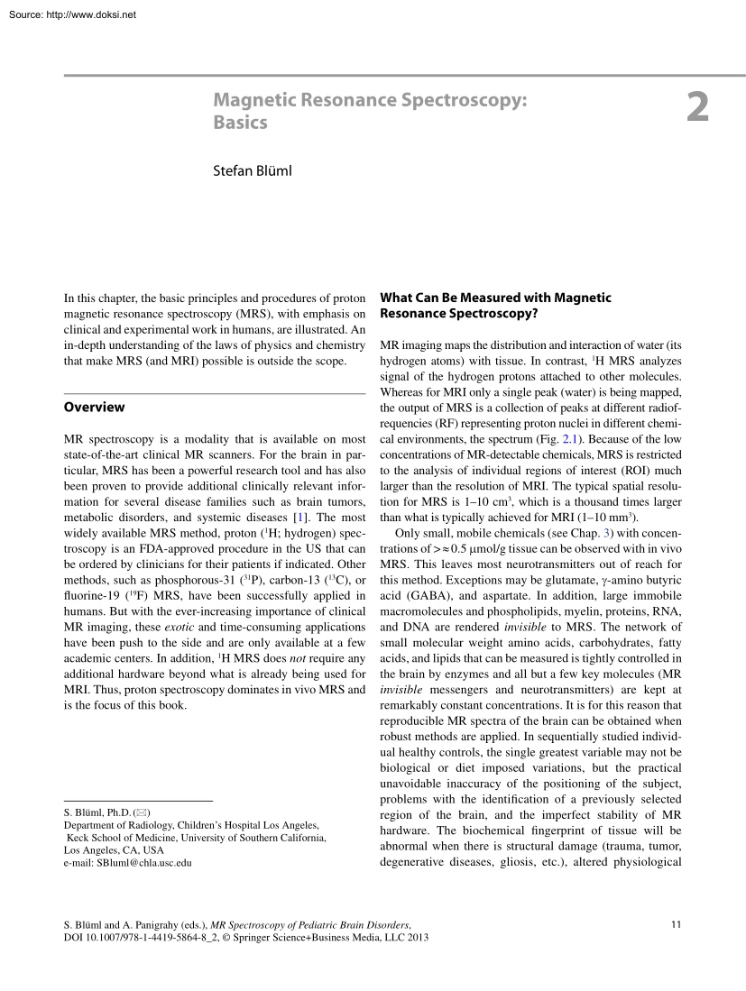
nuclei in different chemical environments, the spectrum (Fig. 21) Because of the low concentrations of MR-detectable chemicals, MRS is restricted to the analysis of individual regions of interest (ROI) much larger than the resolution of MRI. The typical spatial resolution for MRS is 1–10 cm3, which is a thousand times larger than what is typically achieved for MRI (1–10 mm3). Only small, mobile chemicals (see Chap. 3) with concentrations of > » 05 mmol/g tissue can be observed with in vivo MRS. This leaves most neurotransmitters out of reach for this method. Exceptions may be glutamate, g-amino butyric acid (GABA), and aspartate. In addition, large immobile macromolecules and phospholipids, myelin, proteins, RNA, and DNA are rendered invisible to MRS. The network of small molecular weight amino acids, carbohydrates, fatty acids, and lipids that can be measured is tightly controlled in the brain by enzymes and all but a few key molecules (MR invisible messengers and

neurotransmitters) are kept at remarkably constant concentrations. It is for this reason that reproducible MR spectra of the brain can be obtained when robust methods are applied. In sequentially studied individual healthy controls, the single greatest variable may not be biological or diet imposed variations, but the practical unavoidable inaccuracy of the positioning of the subject, problems with the identification of a previously selected region of the brain, and the imperfect stability of MR hardware. The biochemical fingerprint of tissue will be abnormal when there is structural damage (trauma, tumor, degenerative diseases, gliosis, etc.), altered physiological S. Blüml and A Panigrahy (eds), MR Spectroscopy of Pediatric Brain Disorders, DOI 10.1007/978-1-4419-5864-8 2, Springer Science+Business Media, LLC 2013 11 Source: http://www.doksinet 12 Fig. 21 A spectrum is a frequency analysis (=Fourier transform) of the signal that is detected in an MR study. In this case, a

normal gray matter spectrum, acquired from the region of interest (ROI) indicated by the box on the MR image, acquired with a standard PRESS sequence (TE 35ms) at 1.5T is shown The height of a peak is equivalent to the strength of the S. Blüml signal. The position on the x-axis (or chemical shift axis) measures the chemical shift relative to a reference (tetramethylsilane (TMS) at 0 ppm) and can be used to identify chemicals. The water peak would be at 4.7 ppm However, the water peak is suppressed in MRS sequences as it would be several orders of magnitude larger than any of the other peaks conditions (interruption of blood flow, etc.), and biochemical or genetic problems The metabolic fingerprint also varies with the brain region studied There are also normal age-dependent changes during brain development, which are discussed in Chap. 3 Principles of In Vivo Magnetic Resonance Spectroscopy The main ingredient for both MR imaging and spectroscopy is the strong magnetic field (B0)

created by a superconducting magnet. A net magnetization will develop in any tissue brought into the magnet field. The magnetization can be envisioned as a vector pointing, if undisturbed, along the magnetic field For any MR sequence, a radiofrequency pulse, which is an additional time-dependent magnetic field, is used to tip the vector out of its equilibrium position. The magnetization vector will then precess around the equilibrium direction with a characteristic frequency (resonance frequency) Chemical Shift The resonance frequency of the protons is in a first approximation a function of the main magnetic field strength. However, Fig. 22 Left: Hydrogen atom with nucleus (proton) and single electron The electron modifies the magnetic field seen by the proton Right: All protons potentially provide an MR detectable signal. The exact frequency of the signal depends on the molecular structure and the position of the proton in the molecule For example, protons of the CH3 group of

lactate resonate at 1.33 ppm whereas the CH proton resonates at 4.1 ppm the electronic environments of molecules cause a small modulation of the main magnetic field. If the electrons are close to the proton, there is a shielding effect and the proton sees a minimally smaller magnetic field (Fig. 22) This in turn results in slightly different resonance frequencies for protons in different molecules and even for protons in the same molecule but at different positions. Since the chemical structure of molecules determines the electronic environment this shift in the frequency has been named chemical shift. For in vivo MR spectroscopy, analyzing chemical shifts has been the main method for peak assignment. Source: http://www.doksinet 2 Magnetic Resonance Spectroscopy: Basics 13 J-coupling In addition to chemical shifts, the spectrum is also modulated by J-coupling (or scalar coupling). J-coupling is the result of an internal indirect interaction of two spins via the intervening

electron structure of the molecule. The coupling strength is measured in Hertz (Hz) and is independent of the external B0 field strength. J-coupling between the same species of spins, eg, proton and proton is termed homo-nuclear J-coupling whereas J-coupling between different species of spins, e.g, proton and phosphorous is referred to as heteronuclear J-coupling J-coupling results in a modulation of the signal intensity depending on sequence type and acquisition parameters, particularly the echo time (TE, see below). The most prominent example in proton spectroscopy is lactate where there is a 7 Hz strong coupling between the two MR-detectable proton groups. Other molecules with more complex J-coupling patterns are glutamate and glutamine with three J-coupled proton groups. A spectrum of N-acetylaspartate (NAA) is shown in Fig 23 NAA has both uncoupled and J-coupled protons Echo Time and Repetition Time The main contrast mechanisms in MR imaging are T1-saturation, T2-relaxation,

T2*-relaxation, diffusion, and proton density. These properties and the acquisition parameters do affect also the appearance of a spectrum However, each proton in each molecule has its own set of characteristic MR properties. This and the fact that the spectrum itself provides no reference on how a change of an acquisition parameter may affect the spectrum, complicates this issue considerably (In MRI the anatomy provides a reference. For example, bright ventricles in a T2-weighted MRI help to identify other areas of fluid accumulation by the hyperintense signal, etc.) Metabolite resonances may be prominent with one acquisition sequence whereas the peak amplitude is different when another sequence is used despite spectra being acquired from the same ROI (Fig. 24) Therefore, changing sequence parameters or introducing different acquisition sequences should only be done with great caution. Instead, particularly for non-experts, it is important to be consistent and to acquire expertise

with one sequence and one set of acquisition parameters. The most important parameter is the echo time (TE). Indeed, MR spectroscopy can be separated into long TE and short TE methods. As for MR imaging, TE is the time the magnetization is in the transverse plane after an excitation before signal readout. During this time, the signal from each metabolite peak relaxes with its own characteristic T2-relaxation time. In addition, the signal amplitude of protons which are J-coupled is modulated For example, at a Fig. 23 The spectrum of the N-acetyl-aspartate (NAA) molecule is shown (standard PRESS, echo time (TE) 35 ms, 1.5 Tesla) The NAA molecule has protons at different positions. The three protons of the -CH3 group are equivalent and their individual signals add-up and give the prominent peak at 2.0 ppm The other protons attached to carbons of NAA molecule also provide a signal. The protons of the –NH, –CH, and –CH2 are in close proximity in the molecule and do interact via

J-coupling (indicated by dashed arrows in above figure). J-couplings split peaks and modulate the phase of a signal. The result is a more complex pattern of multiple peaks, which can be asymmetric or point downwards. The signal from proton next to the nitrogen atom (amide proton) resonates at approx. 8 ppm Due to rapid exchange with protons from surrounding water molecules, the magnetization disappears quickly and the signal from this proton is very weak characteristic echo time the signal of a metabolite may be inverted (e.g, lactate at TE = 144 ms, Fig 24) Choosing long echo times simplifies spectra because the number of detectable peaks is reduced and the remaining peaks are more readily identified. Historically, long TE (typically TE > 135 ms) has been easier to use in clinical practice because of a flat baseline and because the three peaks (NAA, creatine (Cr), choline (Cho)) can be unequivocally separated. In addition, long TE MRS has been less sensitive to hardware

imperfections (such as eddy currents). More recently, however, significant advances in both hardware and the methods used to analyze spectra have been made. Short TE MRS (TE » 35 ms) allows the detection of an increased number of metabolites and has a signal-to-noise advantage over long TE. Other acquisition parameters that have an impact on the appearance are the repetition time (TR) and the mixing time (TM). TR is the time between each initial excitation of the Source: http://www.doksinet 14 S. Blüml etition time, which more or less simply causes different scaling of peaks. The mixing time TM is the time delay between the second and the third 90° RF pulse in a STEAM sequence. The TE and TM are independent parameters During TM, the magnetization in a STEAM acquisition points along the magnetic file and there is no signal decay due to T2-relaxation. However, during the mixing period there are still processes possible that have an impact on the final appearance of the spectrum

(zero-quantum coherences). Editing Fig. 24 Three single-voxel PRESS spectra of the same ROI acquired with echo times of TE = 288 ms (top), TE = 144 ms (center), and TE = 35 ms (bottom). The spectrum at short TE (35 ms) is more complex and more challenging to interpret However, it also contains more information and is the preferred method particularly for single-voxel MRS. For example, lipids are detectable, there is signal from the amino acids glutamate (Glu) and glutamine (Gln), and myo-inositol is detectable. At TE 144 ms the lactate peak is inverted and this echo time is a good choice when the detection of lactate is particularly important. TE 144 ms is frequently selected for chemical shift imaging (see text for details). At TE 288 ms the lactate signal is in phase again However, at this long echo time, spectra are compromised by low signal to noise and a TE of 288 ms is rarely used on modern MR scanners magnetization. If absolute quantitation is attempted, it is easier to

quantify spectra that were obtained with long repetition times. In this case, knowing the individual T1-relaxation times of all peaks is not as crucial. However, spectra that were acquired with repetition times that are substantially longer than the T1-relaxation times (e.g, TR > 3× T1) are compromised by lower signal-to-noise ratio For that reason, repetition times are generally set to approximately 1–15 times the T1-relaxation times of metabolites. In contrast to TE, the overall appearance of spectra does change little with the rep- Editing techniques exploit unique homonuclear (or heteronuclear) J-coupling properties of molecules. Many editing sequences utilize the fact that in an echo sequence the phase of J-coupled spins is modulated during the echo delay. A series of spectra acquired with different echo times each may allow the separation and identification of overlapping signals from different molecules due to their different J-modulation. Metabolite editing confers some

specificity on the process of peak identification in high-resolution NMR techniques but has so far contributed little new information to in vivo human brain studies. Practical in vivo sequences have been proposed by Ryner et al. [2] and Hurd et al [3] and tested in human subjects. While many creative editing sequences from high-resolution NMR are available in the literature, in practice, signal-to-noise limitations preclude their use in vivo. For example, zero-quantum filter for lactate editing is accomplished with a 2:1 signal loss; simple short-echo time sequences without metabolite-specific editing may work just as well. Recent examples of successful in vivo editing include GABA [4, 5] and b-hydroxy butyrate [6]. Data Acquisition Planning a Magnetic Resonance Spectra Planning and performing an MRS study is complex and requires extra diligence when compared with the planning of an MRI study. All modern MR scanners allow straightforward planning of MR imaging studies where the

operator selects enough slices to cover the whole head and thus all areas of interest. With most acquisition parameters conveniently stored in ready-to-go protocols there is little that can go wrong. In contrast, quality control at the time of data acquisition is essential for MR spectroscopy. For MR spectroscopy, the operator needs to select the correct region of interest and may need to adjust scan parameters. Even in case of a focal lesion, such as a tumor, it might be necessary to pick the correct part of the tumor (e.g, avoiding bleeds or Source: http://www.doksinet 2 Magnetic Resonance Spectroscopy: Basics calcifications, selecting more cellular parts instead of a necrotic center, staying away from the skull, etc.), adjust the size of the region of interest, and the required scan time. Even with volumetric chemical shift imaging where many spectra from different locations are acquired simultaneously (CSI, discussed in more detail below) it is not possible to cover more than

a part of the brain. Acquisition Methods: Single-Voxel Versus Chemical Shift Imaging Single-Voxel Magnetic Resonance Spectroscopy Single-voxel (SV) MRS measures the MR signal of a single selected region of interest whereas signal outside this area is suppressed. For single-voxel MRS, the magnetic field and other parameters are optimized to get the best possible spectrum from a relatively small region of the brain. Manufacturers generally provide PRESS (Point Resolved Spectroscopy) [7, 8], STEAM (Stimulated Echo Acquisition Mode) [9], and ISIS (Image Selected In Vivo Spectroscopy) [10]. These sequences differ in how radiofrequency pulses and so-called gradient pulses are arranged in order to achieve localization. It is beyond the scope of this chapter to discuss details about localization methods and the interested reader is referred to the above-mentioned publications. ISIS is based on a cycle of eight acquisitions, which need to be added and subtracted in the right order to get a

single volume. ISIS is considerably more susceptible to motion than STEAM or PRESS and is mostly used in heteronuclear studies, where its advantage of avoiding T2-relaxation is valuable. For 1H MRS, however, ISIS has fallen out of favor. Both, PRESS and STEAM do not require the addition or subtraction of signals to achieve localization and are thus more robust. PRESS utilizes one 90° and two 180° slice selective pulses along each of the spatial directions and generates signals from the overlap in form of a spin echo. At the same echo time, PRESS has the advantage over STEAM that it recovers the full possible signal and is therefore the method of choice for applications where signal to noise (S/N) is crucial. Since S/N is always crucial in MR, PRESS appears to be the overall winner among the competing localization techniques. STEAM utilizes three 90° slice selective pulses along each of the spatial directions. Signal, in form of a stimulated echo, from the overlap is generated STEAM

allows shorter echo times than PRESS partially compensating for lower S/N. Secondly, the RF bandwidth of 90° pulses is superior to the bandwidth of 180° pulses utilized by PRESS. STEAM is therefore an alternative to PRESS when short echo times, minimal chemical shift artifacts, and robustness are of concern. 15 2D or 3D Chemical Shift Imaging With chemical shift imaging (CSI) approaches, multiple spatially arrayed spectra (typically more than 100 spectra per slice) from slices or volumes are acquired simultaneously. Other terms used for CSI are spectroscopic imaging (SI) and MR spectroscopic imaging (MRSI). Slice selection can be achieved with a selective RF pulse as for MR imaging. CSI encodes all spatial information into the phase of the magnetic resonance signal. In contrast to standard 2D MR imaging where one spatial dimension is phase encoded while the second dimension is frequency encoded, data acquisition is performed in the absence of a frequency-encoding gradient so that

the chemical shift information can be retained. Due to the phase encoding, many spectra from a slice or from a 3D volume can be acquired simultaneously, and CSI is an excellent technique to obtain metabolic maps (Fig. 25) When it is desired to limit the region of interest to a smaller volume, e.g, to avoid bone and fat from the skull, CSI is usually combined with PRESS, STEAM, or ISISbut with a significantly larger volume selected than for single-voxel MRS. CSI is a very efficient method to acquire information from different parts of the brain. An important feature is that within the examined volume of interest, any ROIs can be selected retrospectively by a process termed voxel-shifting. When to Use What Method? Despite evidence for the value of MRS in clinical practice and technical improvements, the application of MR spectroscopy is still hampered by its technically challenging nature. MR spectroscopy is prone to artifacts and processing and interpretation is complex and requires

expert knowledge. For MRS to be used in clinical research and practice, standardized acquisition and processing methods need to be employed, easy to follow rules for quality-control applied, and results need to be presented and documented in a timely fashion to have an impact on clinical decision making. Studies should be designed not only to address basic medical or biological questions but also keeping the available resources in mind. Bulky CSI acquisitions with the need to review and interpret hundreds of spectra may require a skilled MR spectroscopist. Therefore, most new investigators will do better in the beginning by employing a singlevoxel method This ensures high quality of individual spectra Single-voxel MRS performs more robustly when short echo times are selected. Employing a short echo time ensures high S/N of spectra and minimizes the signal loss of fast decaying peaks of metabolites such as myo-inositol, glutamate, and glutamine. Therefore, for single-voxel studies,

short echo time PRESS (TE £35 ms) or STEAM (TE £30 ms) are recommended. However, single-voxel MRS is not a practical Source: http://www.doksinet 16 S. Blüml Fig. 25 (a) 2D CSI of a 3-year-old boy with a posterior fossa astrocytoma The data were acquired with a PRESS sequence with a repetition time (TR) of 1.0 s, TE = 35ms, field of view = 160 bmm, 20 × 20 phase encoding steps, slice thickness = 8 mm, and two averages resulting in a nominal voxel resolution of 0.5 cc Acquisition time was 133 min The large boxes indicate the excited volume; smaller boxes indicate anatomical locations of individual spectra. (b) Shown is a 2D CSI of a child with a glioblastoma after radiation therapy. The box on the left image indicates the area from which spectra were acquired. Instead of displaying individual spectra, on the right, the results of the spectroscopy study are displayed as a color map. In this case, areas with increasing prominent choline relative to creatine (tCho/Cr) were colored

hot yellow to red whereas areas with decreasing tCho/Cr are displayed in green and blue. Acquisition parameters were similar to those used in Fig 25a approach when maps of the distribution of chemicals within the brain are the goal. The investigator who wants to study many different brain regions or who needs to understand the spatial distribution of metabolites in an efficient matter will need to employ CSI. However, it should be noted that the added information available from CSI acquisitions sampling larger volumes might be compromised by poorer magnetic field homogeneity resulting in less well-defined peaks and nonuniform water suppression. In practice, it is more important to know which parameters and how various parameters influence S/N. Signal-to-Noise Ratio Insufficient signal-to-noise ratio (S/N) is the most significant challenge of in vivo MRS and its main limitation in clinical practice! It is not required for users of MRS to become experts in the discussion of how to

best measure absolute S/N. The definition and the measurement of absolute S/N depend on acquisition parameters and steps involved in preprocessing of the data. For our purposes, S/N is the ratio between the amplitude of a resonance and the amplitude of random noise observed elsewhere in the spectrum (Fig. 26) Rules (and Qualifiers) for Signal-to-Noise Ratio 1. To improve the S/N by a factor of two, four times the acquisition time is necessary. To have a three-fold signal increase, nine times the acquisition time is necessary. 2. But: There are practical limitations to increasing the scan time: If a scan exceeds the time a patient can hold still, nothing will be gained. Patient movements may degrade the quality of a study and the uncertainty of the location and thus the composition of the tissue enclosed in the region of interest compromising the interpretation. Hardware instabilities also take away S/N in scans that take a long time. From our experience, we believe that the

acquisition time of a single scan should not exceed 20 min. We acknowledge, however, that under circumstances when a patient is very cooperative scans that last longer can be carried out. More typical and practical acquisition times that are well tolerated are 3–6 min. 3. S/N scales with the volume; half the volume gives half the S/N, doubling the volume doubles the S/N. This is Source: http://www.doksinet 2 Magnetic Resonance Spectroscopy: Basics 17 Fig. 26 This example illustrates that the S/N of a spectrum needs to be considered before drawing any conclusions. The same simulated spectrum with peaks with amplitude ratios of 4:2:1 is shown in (a–d) The hypothetical case of the spectrum with unlimited S/N is shown on the top left (a). In the next step random noise at a moderate level was added and peaks with approximate ratios of 4:2:1 are still observed. Spectra (c) and (d) are two simulations with twice the noise added, respectively. The original amplitude ratios are not

reproduced and the spectra can only be interpreted qualitatively. Indeed, peaks b and c have become undetectable in simulation (d) because the signal is proportional to the volume of the selected region. On the other hand, the noise is produced by the entire tissue within the sensitive volume of coil. The noise does not change with selecting different ROIs. (As the noise level in a study is constant, it is possible to compare two spectra that were acquired from different but equally sized ROIs to obtain information about absolute concentrations in both spectra: Scale both spectra such that the noise level is the same in both spectra. Compare the amplitude of the peaks CAVEAT: This does not work if the linewidths of the peaks of the two spectra are substantially different.) 4. To compensate for a volume reduction by a factor of two the scan time needs to be increased by a factor of four. 5. But: A good shim (= process of optimizing the homogeneity of the magnetic field at the region of

interest) improves the S/N. The area of a resonance line is constant Therefore, by improving the shim and narrowing the width and increasing the amplitude of a resonance line the S/N can be improved. Generally, better shims are achieved for smaller ROIs. Thus, increasing the ROI size does not guarantee a linear increase in S/N. Similarly, decreasing the ROI might not result in a linear reduction of S/N. 6. But: Another finer point is the shape of a voxel A cubic voxel can be shimmed better than an odd shaped voxel (very long in one direction and short in another direc- tion). Therefore, ROIs that are closest to a cubic shape have the best S/N among rectangular ROIs with the same volume (spheres would be even better). The S/N decreases with increasing echo times (TE) due to the T2-decay of the signal. Shorter repetition times (TR) cause T1-saturation. This does not necessarily reduce the S/N because more averages can be packed into the same acquisition time. T1 and T2 relaxation times

vary with metabolites and field strength. In respect to S/N, the shortest possible TE is the best choice (but there are other important considerations). There is no best TR At 1.5T a TR between 1 and 3 s is a good choice; at 3 T a TR between 2 and 5 s is appropriate. If a user wants to acquire several spectra, choosing a large CSI box to cover all regions of interest is more efficient than measuring individual spectra with a singlevoxel MRS. On the other hand, spectral quality of CSI is often compromised when single-voxel works fine. With equal TR and TE, a PRESS sequence provides twice the S/N of a STEAM sequence. Increasing the field strength will improve the S/R. Moving from 1.5 to 3 T scanners doubles the magnetization In practice this does not result in a doubling of the S/R. This is because at 3 T T1-relaxation times are longer (=larger saturation effects), T2-relaxation times are shorter (faster signal decay), and the homogeneity of the magnetic field of 3T magnets does not

reach the 7. 8. 9. 10. Source: http://www.doksinet 18 homogeneity achieved at 1.5 T Still, an S/R improvement of at least 50% can probably be achieved with modern 3 T systems. 11. Radiofrequency coils that are optimized (as small as possible without causing inhomogeneous excitation) will provide better S/N when compared with large coils. Selecting the Region of Interest On modern MR scanners, MR spectroscopy sequences are fully integrated into protocols and there is little difference between an MRI and an MRS study for patients. For the operator, on the other hand, MRS requires an additional important step. Using an image just obtained, a region of interest (ROI) is selected from which the MR spectrum is obtained. Indeed, selecting an appropriate ROI is probably the most crucial part of an MR spectroscopy study. This is particularly important for diseases with focal lesions. Not only needs the operator decide on the appropriate location, but also other factors such as size (in

all three dimensions), number of averages required to obtain a spectrum of sufficient quality, minimizing partial volume with surrounding tissue, avoiding proximity to skull/bone/air transitions (negatively impact quality), avoiding blood and calcifications, and limiting the amount of cerebrospinal fluid (has no metabolites) need to be taken into consideration. Accuracy in prescribing a region of interest (and proper documentation for longitudinal studies!) is of great importance in particular for single-voxel MRS studies. It is therefore recommended to study brain regions where MRS works and where normal MRS data are readily available for comparison. Two very popular choices are parietal white matter and occipital gray matter which have been studied frequently with single-voxel MRS. Frontal white matter and basal ganglia, historically technically more challenging, are also frequently studied brain regions How to Acquire Good Quality Spectra Acknowledging that good is a relative term,

below are a few suggestions on how to ensure that the quality of an MRS study is close to what can be achieved under optimum conditions. In order to acquire good spectra, for MRS the magnetic field within the region of interest is further refined in a process called shimming. Whereas in the early days of MRS a skilled spectroscopist would perform this task, today’s scanners all have automated procedures that are generally equally good, faster, and more objective. Indeed, shimming as well as other scanner adjustments, such as transmitter and receiver gain setting, water suppression, is now all by default incorporated into the sequence. The user, after selecting the S. Blüml ROI, merely pushes a button and awaits the completion of the study. Good spectra are obtained if the ROI was not selected too small or too large, was not placed over areas of bleeds or calcifications, and away from tissue/bone/air transitions. When the voxel size is too small spectra of inadequate S/N are

obtained It is recommended to use approximately 10 cc at 1.5T for a single-voxel examination with PRESS with 128 averages. Depending on the biological/clinical question, it is possible to have smaller (or larger) ROIs. For example, if the question is whether there is elevated choline in the ROI, but accurate quantitation is not required, a smaller voxel will do. Other applications, for example phenylalanine in phenylketonuria (PKU), require the measurement of metabolites that are at very small concentrations. In this case, the ROI needs to be larger Bleeds and, to a lesser extent, calcifications distort the magnetic field resulting in broad lines and poor water suppression compromising spectral quality. Similarly, placing the ROI on an area that contains a mixture of tissue, skin, bone, and air will result in poor spectra because the magnetic field cannot be adjusted very well. In summary, careful placement and proper selection of the size of the ROI are the only remaining hurdles for

obtaining good quality spectra on modern MR scanners. While experience is useful, this task does certainly not require an MR spectroscopist. Processing and Quantitation In the early days of spectroscopy, a file that contains the raw result of the spectroscopy study would be stored somewhere on the computer that controls the MR scanner. That file would then be typically copied to an off-line computer for further processing using often custom-designed software. The basic processing steps are: • Linebroadening: Linebroadening is a filtering process by which the measured signal is multiplied with a function that effectively improves the S/N of a spectrum at the cost of reduced spectral resolution. Alternatively, the filter function improves spectral resolution (negative linebroadening) at the cost of reduced S/N. • Fourier transform: A Fourier transform is a mathematical operation that decomposes the measured signal in the time domain to its frequencies. • Phasing: Due to hardware

settings and sequence timing following the Fourier transform, a mixture of absorption and dispersion signals is observed in the spectrum. Spectrum analysis and quantitation is performed on the pure absorption signal, which needs to be extracted by a phase correction procedure. Most modern MR scanners provide semi- or fully automated FDA approved scripts that can be used for processing. When using those, it is highly recommended to be method- Source: http://www.doksinet 2 Magnetic Resonance Spectroscopy: Basics ological and refrain from experimenting with the processing parameters. Phasing and linebroadening do have an impact on the appearance of the spectrum and thus on the interpretation. Users with consistent processing parameters have an advantage particularly when longitudinal studies are being performed. Recently, sophisticated processing software packages such as LCModel or MRUI [11, 12] have significantly improved automatic assignment and quantitation of metabolites in in

vivo MR spectra. Processing of spectra is accomplished by fitting in vivo spectra to linear combinations of typically 15–20 measured or simulated model spectra of metabolites. This list of metabolites includes the major metabolites (e.g, NAA, Cr, Cho, mI) but also less prominent metabolites (e.g, glucose (Glc), or taurine (Tau)) These software packages are particularly appropriate for investigators who work with scanners from different vendors as they ensure equivalent processing and thus comparability. Albeit, these software packages are clearly superior to manufacturer provided solutions, they are not FDA approved and are thus more frequently used in research settings. Often a neglected step is the proper documentation (preferable on three orthogonal images) of the location of the ROI. If the location of the ROI is not documented the MRS study is not complete. Unfortunately, manufactures do not appreciate the need for good (and automatic!) documentation and the user is settled to

use the various, sometimes not intuitive, manual tools available. 19 employed strategy for absolute quantitation is to acquire the water signal of the brain in the region of interest and measure (or assume) the water content of tissue. This can then be used as an internal concentration reference. For example, the water signal of tissue with a water content of 80% corresponds to a concentration of 55 mol/l × 80% = 44 mol/l. Use of the water signal as an absolute concentration reference eliminates several sources of error, such as differences in voxel size, total gain due to coil loading, receiver gains, hardware changes, etc. However, often the water content, in particular in pathology, is unknown. Therefore, other quantitation methods, using for example an external reference, have been suggested. Absolute quantitation of CSI data sets is challenging. Whereas for single-voxel MRS sampling the water signal does not add more than a few seconds to the scan time, the situation is

different for CSI. To obtain the reference water signal for each region of interest the acquisition of an additional CSI data set with time consuming 2D or 3D phase encoding is necessary. An alternative approach is to skip the extra scan and use the metabolite signal of normal tissue, distant from a focal abnormality, as internal reference. This approach has problems when metabolic changes in apparently normal appearing tissue cannot be ruled out. For a more detailed discussion of quantitation methods, the interested reader is referred to [13, 14]. Miscellaneous Absolute Quantitation Safety For MR spectroscopy to become an accepted tool for research and clinical application, the information needs to be quantified and condensed in a fashion that allows the nonexpert user to draw adequate conclusions in a timely fashion. The natural parameters appear to be concentrations of metabolites in moles per unit volume, wet weight, or dry weight linking MRS with existing norms of biological

chemistry. However, more common are peak ratios by which the signal intensity of one metabolite is expressed as a fraction of another one. Cr has often been used as an internal reference and metabolite ratios relative to Cr are reported. This was based on the assumption that the Cr pool is relatively constant in normal and diseased brain. However, this is not always the case and might be misleading. In particular, tumors may have quite different levels of Cr than normal tissue and ratios may be quite misleading. Even the structurally intact-looking brain might have altered concentrations of creatinefor example, the developing brain or under in hypo- and hyper-osmolar conditions. Therefore, although in many instances ratios provide important information, absolute quantitation is the preferred method. One commonly Three different magnetic fields are applied in MRS: • Static magnetic field B0 • Gradient fields for localization purposes • RF fields to excite the magnetization These

static fields are generally remarkably safe, with no known biological hazards. Fast switching gradients have been considered as associated with risk and nerve stimulation. While there exist exotic techniques such as echo planar spectroscopic imaging (EPSI), the vast majority of MRS techniques switches gradients a magnitude slower than routinely applied in MR imaging. Prolonged irradiation of RF is identified as hazardous to the extent that energy is deposited in the human head. But, again, MRS, when compared with MRI uses only few RF pulses and excessive RF deposition is not a problem in 1H MRS. Magnetic Resonance Spectroscopy at 3T The main benefit of higher field strength for MRS is the increased SNR. MR spectroscopy also benefits from the Source: http://www.doksinet 20 Fig. 27 Shown are spectra from the same patient and ROI (white box in MRI) acquired at 1.5 T and at 3 T Both spectra cover the same chemical shift range (0–4 ppm) However, if the x-axis would be measured in

hertz, the 1.5 T spectrum would cover 260 Hz (4 ppm = 4 × 65 Hz at 1.5 T) whereas the 3 T spectrum would cover 520 Hz (4 ppm = 4 × 130 Hz at 3 T). The acquisition times are comparable Note, that the 3 T spectrum has considerable better SNR (lower level of random signal outside increased spectral resolution. Essentially, when moving from 1.5 to 3 T, a spectrum is being stretched along the chemical shift (x-axis) by a factor of two (Fig. 27) A disadvantage of the higher field strength is the increased chemical shift artifact. This problem arises from the different frequencies of the resonances associated with various chemical structures. When a gradient is applied to a sample containing chemically shifted species, there will be a displacement of the sensitive volume for each of the different species. The bandwidth of the RF pulse, with respect to the chemical shift range of the chemical structures, sets the percentage of overlap one can expect. Since at 3 T the chemical shift range is

two times larger than at 1.5 T there is less (half) overlap (or more chemical shift artifact) at 3 T when the same RF pulse is used for excitation. Increasing the bandwidth of the RF pulse reduces chemical shift artifacts. In addition, whereas the main singlet peaks NAA (2.0 ppm), Cr (3.0 ppm), Cho (32 ppm) remain singlets at 3 T, the spectral pattern of other metabolites may change. Unfortunately, for some metabolites, such as taurine, detectability does not improve or may even decrease at higher field (Fig. 28) S. Blüml peaks). In this case the improvement may be exaggerated as the 15 T spectrum was acquired on an old system whereas the 3T spectrum was acquired on a state-of-the-art scanner with a smaller head coil. Also, note that while the creatine and choline singlets are rendered unchanged, the appearance of the myo-inositol signal (mI) is different for the two field strength (see also Fig. 2–8) Fig. 28 Spectra of chemicals are generally different at different field

strength as illustrated here for taurine and myo-inositol. Both spectra were acquired from model solutions with a PRESS TE 35 ms sequence. Changes in patterns need to be taken into consideration when comparing spectra acquired at different field strength Finally, one has to consider that T1-saturation and T2-relaxation of metabolites are different at 1.5 T and 3 T To complicate matters, relaxation properties for different metabolites do not change equally. Still, the benefits of improved SNR and spectral resolution at 3 T probably outweigh the disadvantages. Using a 3 T system, when available, is thus recommended Source: http://www.doksinet 2 Magnetic Resonance Spectroscopy: Basics 21 Basic Questions/Answers Often questions like “what is the smallest voxel you can measure?, how do I know that the signal-to-noise ratio is sufficient?, how do I know it is an artifact?”, etc. are asked These questions do have in common that there is no definitive answer and, consequently, no

definitive answer can be provided in this book. Instead, below, we will try to elucidate a spectroscopist’s point of view. Obviously, even within the MRS community there are different opinions and approaches. Thus, it is hereby disclosed that what is written and explained below is biased by the editors’ opinions. What is the smallest voxel that can or should be measured? What is the minimum S/N needed for a study to be conclusive? For global disorders, there is no need to push for the smallest possible voxel. Otherwise, for focal processes, there isno surpriseno definitive answer to these questions. The approach depends on how much time an investigator is willing to invest and on the importance of the question that is being asked. It also depends on the quality of the shimming and the shape of the voxel. We advise against beginning a study with an acquisition of a spectrum from a very small voxel. Should the result only show random noise it would be unclear whether this is due to

insufficient S/N or a feature of the tissue and valuable scan time has been wasted. A better approach might be to acquire a spectrum from a ROI large enough for the investigator to detect the major peaks of a spectrum. In a second step, the investigator can then reduce the voxel size and increase the scan time taking into account the rules given above and judging from the relative peak heights and noise level of the already acquired spectrum. Obviously, for the interpretation, the partial volume of surrounding tissue needs to be considered. To provide a number: We advice to select ROIs smaller than 1 cc only in extreme situations for single-voxel MRS. For CSI we advice against a resolution better than 0.5 cc If a spectrum is very noisy, how do I know whether this is due to technical problems or whether presents true biology (e.g, hypocellularity, necrosis, etc)? Looking at the noisy spectrum itself may not help to answer this question. Even before an MRS acquisition, MR and CT images

(if available) should be inspected for bleeds and for calcifications. These areas should be avoided to the extent possible. Check the size of the ROI If the volume is less than 1cc and the scan time has not been prolonged substantially, low S/N is the problem. In addition, it should be ruled out that the patient moved considerably during a scan by, for example, comparing MRI studies before and after the MRS study (another reason not to do conduct MRS studies at the very end of an examination). Distortions on MRI may indi- Fig. 29 The partial volume of surrounding normal tissue is easily underestimated in MRS. For example, the volume of spherical lesion is 4/3 r3p where r is the radius of the lesion. The volume of a cubic ROI enclosing the lesion is 8 r3. That means that in this case the partial volume is approximately 50% The resulting spectrum will show a mixed pattern with approximately equal contributions of metabolites from the lesion and from surrounding tissue cate a technical

artifact caused by braces (quite common in children) or by other magnetic parts. If this does not explain a bad spectrum there is more information that should be reviewed. While metabolites concentrations might be too low to produce peaks in a spectrum there is always enough signal from water. Unfortunately, some manufacturers do not routinely acquire a water spectrum or store it for convenient review. However, all scanners use water for the shimming procedure and the numeric result of the shimming can generally be reviewed. If a spectrum was acquired from a standard-sized voxel and the final shim was within the normal range, the absence of metabolites in the spectrum means that metabolites are low. Good shims are 01 ppm or less (6 Hz or less at 1.5 T and 12 Hz or less at 3 T) If shims are 015 ppm or worse data should be interpreted very carefully as the absence of certain metabolic features is likely explained by the low quality of the study. How much partial volume do I have? For the

interpretation of an MRS study, a realistic assessment of partial volumes is an absolute prerequisite! For global disorders or any study where standardized regions are examined, partial volumes are a minor problem. Consistency in the methods and accuracy in the placement of a voxel ensure reproducible findings. Partial volume effects are, however, a major challenge for focal processes. A typical scenario is a small focal lesion that is being studied with MRS. As is illustrated in Fig 29, it is easy to underestimate the extent of partial volume. What is the chemical shift artifact? The net result of the chemical shift artifact is that the ROIs for the various metabolites in a spectrum do have significant overlap but are not identical. The problem of chemical shift Source: http://www.doksinet 22 S. Blüml Fig. 210 Spectra obtained from a patient with seizures (top trace) and a patient with hepatic encephalopathy, a disorder associated with increased glutamine (bottom trace). Spectra

of model solutions of glutamate and glutamine are shown for comparison (middle traces). Note, that in the hepatic encephalopathy spectrum the pattern of the b, g-Glx region follows the glutamine signal whereas in the seizure case the pattern is more consistent with glutamate. All spectra: Singlevoxel PRESS, TE 35 ms, 15 T artifacts arises from the different frequencies of the signal that is observed in MRS. When a gradient for localization is applied there will be a displacement of the sensitive volume for each of the different species. The bandwidth of the RF pulse, with respect to the chemical shift range of the chemical structures, sets the percentage of overlap one can expect. Increasing the bandwidth of the RF pulse reduces chemical shift artifacts. Chemical shift artifacts are a bigger problem at higher field strength. Because most MRS sequences are already optimized, there is not much that can be done to reduce chemical shift artifacts. Chemical shift artifacts can cause

problems for MRS of focal lesions. For example, lipids are important markers of tumor malignancy as the lipid signal indicates membrane breakdown and necrosis. The specificity of lipid signal is compromised when the ROI for the spectroscopy is close to skull/bone and lipid signal from the skull can be misinterpreted as signal from the lesion. I see in the spectrum an unusual peak/signal. Is it real? Over the years, spectroscopists have been taught by experience what can and what cannot be observed with in vivo MRS in the human brain. Still, occasionally new peaks are discovered. The number of unusual peaks observed with in vivo spectroscopy has dropped significantly over time. This is mainly a result if greatly improved hardware and software and thus less artifacts being confused with real signal. If a patient is still on the scanner, a second spectrum should be acquired. If a global disorder is expected, a different brain region should be selected. In case of a focal lesion, a

slightly different ROI should be selected. In addition, a spectrum with a different echo time should be acquired if possible. Scanner stability: Are there Monday morning and Friday afternoon peaks? Brain metabolism is very well regulated and MRS is remarkable stable. There are no Monday morning or Friday afternoon peaks. Exceptions are glucose, which can increase/ decrease with plasma glucose. Can glutamate and glutamine be separated at 1.5 T? It depends. Due to their similar chemical structures, glutamate and glutamine form complex and partially overlapping resonances in 1H spectra. However, although the individual spectra of glutamate and glutamine are similar, they are not identical (Fig. 210) That means, that the quality of a spectrum (linewidth and signal to noise) determines how well the contribution from these two metabolites can be distinguished. Hypothetically, with unlimited signal to noise, perfect separation is possible and a categorical claim that glutamate and glutamine

cannot be separated at 1.5 T is wrong Still, it needs to be acknowledged that only under the best circumstances glutamate and glutamine can be quantified in Source: http://www.doksinet 2 Magnetic Resonance Spectroscopy: Basics 23 example, a peak at around 2.45 ppm Spectra obtained from tissue with high levels of glutamine will show this peak whereas this signal is much less prominent in a situation where glutamate concentration exceeds glutamine. So even without sophisticated software, just by careful inspection of the spectra, it is possible to make a qualitative statement about glutamate and glutamine. But there is an important caveat: Spectra need to be of high quality with the random noise signal below the signal amplitudes of glutamate and/ or glutamine. References Fig. 211 Spectra obtained from a patient with a normal MRI and unremarkable follow-up (upper trace) and a patient with acute liver failure (middle). A spectrum of a model solution of glutamine is shown for

comparison (bottom). Note that in the patient with liver failure the signal at around 2.45 pm is consistent with elevated glutamine Advanced processing with LC Model suggested that glutamine concentration in the liver failure patient is at least three times higher than glutamate. In the control, glutamate concentrations are approximately three times higher than glutamine individual patients at 1.5 T Also, it is advised to use sophisticated software, such as LCModel (Provencher 1993) that fits all metabolite resonances simultaneously and provides a measure of the reliability of the analysis (so called Cramer– Rao lower bounds). A prerequisite is to use short TEs to minimize signal decay. Special acquisition methods (editing) can be used to improve the separation. However, these methods are not widely available, are compromised by longer acquisition times, and require extra expertise. Separation of glutamate and glutamine improves greatly at 3 T. Can we distinguish between glutamate

and glutamine in spectra acquired at 3 T in individual patients? Tentatively yes. At 3 T, the glutamate and glutamine signals can be much better distinguished than at 1.5 T As illustrated (Fig 211), for PRESS TE 35 ms, glutamine has, for 1. Ross BD, Bluml S Neurospectroscopy In: Greenberg JO, editor Neuroimaging second edition; a companion to Adams and Victor’s principles of neurology. New York: McGraw Hill; 1999 p. 727–73 2. Ryner LN, Sorenson JA, Thomas MA Localized 2D J-resolved 1H MR spectroscopy: strong coupling effects in vitro and in vivo [published erratum appears in Magn Reson Imaging 1995;13(7):1043]. Magn Reson Imaging. 1995;13(6):853–69 3. Hurd RE, Gurr D, Sailasuta N Proton spectroscopy without water suppression: the oversampled J- resolved experiment. Magn Reson Med. 1998;40(3):343–7 4. Rothman DL, Petroff OA, Behar KL, Mattson RH Localized 1H NMR measurements of gamma-aminobutyric acid in human brain in vivo. Proc Natl Acad Sci USA 1993;90(12):5662–6 5.

Hetherington HP, Newcomer BR, Pan JW Measurements of human cerebral GABA at 4.1 T using numerically optimized editing pulses Magn Reson Med. 1998;39(1):6–10 6. Shen J, Novotny EJ, Rothman DL In vivo lactate and beta-hydroxybutyrate editing using a pure-phase refocusing pulse train Magn Reson Med. 1998;40(5):783–8 7. Bottomley PA, Inventor Selective volume method for performing localized NMR spectroscopy. US patent US patent 4 480 2281984. 8. Bottomley PA Spatial localization in NMR spectroscopy in vivo Ann N Y Acad Sci. 1987;508:333–48 9. Frahm J, Merboldt K, Haenicke W Localized proton spectroscopy using stimulated echos. J Magn Reson 1987;72:502–8 10. Ordidge RJ, Connelly A, B Lohman JA Image-selected in-vivo spectroscopy (ISIS). A new technique for spatially selective NMR spectroscopy. J Magn Reson 1986;66:283–94 11. Provencher SW Estimation of metabolite concentrations from localized in vivo proton NMR spectra. Magn Reson Med 1993; 30(6):672–9. 12. Naressi A, Couturier

C, Devos JM, et al Java-based graphical user interface for the MRUI quantitation package. MAGMA 2001; 12(2–3):141–52. 13. Kreis R Quantitative localized 1H MR spectroscopy for clinical use. Prog NMR Spectroscopy 1997;31:155–95 14. Danielsen ER, Henriksen O Absolute quantitative proton NMR spectroscopy based on the amplitude of the local water suppression pulse. Quantification of brain water and metabolites NMR Biomed 1994;7(7):311–8