Informatika | Információelmélet » Ramesh Johari - Adaptive learning

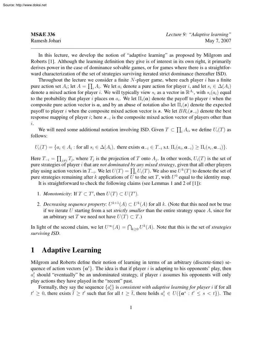
Source: http://www.doksinet MS&E 336 Ramesh Johari Lecture 9: “Adaptive learning” May 7, 2007 In this lecture, we develop the notion of “adaptive learning” as proposed by Milgrom and Roberts [1]. Although the learning definition they give is of interest in its own right, it primarily derives power in the case of dominance solvable games, or for games where there is a straightforward characterization of the set of strategies surviving iterated strict dominance (hereafter ISD). Throughout the lecture we Q consider a finite N -player game, where each player i has a finite pure action set Ai ; let A = i Ai . We let ai denote a pure action for player i, and let si ∈ ∆(Ai ) denote a mixed action for player i. We will typically view si as a vector in RAi , with si (ai ) equal to the probability that player i places on ai . We let Πi (a) denote the payoff to player i when the composite pure action vector is a, and by an abuse of notation also let Πi (s) denote the expected

payoff to player i when the composite mixed action vector is s. We let BRi (s−i ) denote the best response mapping of player i; here s−i is the composite mixed action vector of players other than i. Q We will need some additional notation involving ISD. Given T ⊂ i Ai , we define Ui (T ) as follows: Ui (T ) = {ai ∈ Ai : for all si ∈ ∆(Ai ), there exists a−i ∈ T−i s.t Πi (ai , a−i ) ≥ Πi (si , a−i )} Q Here T−i = j6=i Tj , where Tj is the projection of T onto Aj . In other words, Ui (T ) is the set of pure strategies of player i that are not dominated Q by any mixed strategy, given that all other players play using action vectors in T−i . We let U (T ) = i Ui (T ) We also use U k (T ) to denote the set of pure strategies remaining after k applications of U to the set T , with U 0 equal to the identity map. It is straightforward to check the following claims (see Lemmas 1 and 2 of [1]): 1. Monotonicity: If T ⊂ T ′ , then U (T ) ⊂ U (T ′ ) 2.

Decreasing sequence property: U k+1 (A) ⊂ U k (A) for all k (Note that this need not be true if we iterate U starting from a set strictly smaller than the entire strategy space A, since for an arbitrary set T we need not have U (T ) ⊂ T .) T In light of the second claim, we let U ∞ (A) = k≥0 U k (A). Note that this is the set of strategies surviving ISD. 1 Adaptive Learning Milgrom and Roberts define their notion of learning in terms of an arbitrary (discrete-time) sequence of action vectors {at }. The idea is that if player i is adapting to his opponents’ play, then ati should “eventually” be an undominated strategy, if player i assumes his opponents will only play actions they have played in the “recent” past. Formally, they say the sequence {ati } is consistent with adaptive learning for player i if for all ′ t ≥ 0, there exists t ≥ t′ such that for all t ≥ t, there holds ati ∈ U ({as : t′ ≤ s < t}). The 1 Source: http://www.doksinet sequence

{at } is consistent with adaptive learning if {ati } is consistent with adaptive learning for all players i. In the definition, the value t′ defines a “recent past”, and the value t defines a reasonable “adaptation period”. This is significantly more general than fictitious play: there is no requirement that every play of player i should be undominated given the entire past history. Rather, after looking at the play of his opponents, player i should eventually play strategies that are undominated, when ignoring strategies of players j 6= i that have not been played for a sufficiently long time. As Milgrom and Roberts note, schemes like fictitious play, best response dynamics, and even Bayesian learning are all consistent with adaptive learning. To get a feel for this, we consider a class of learning algorithms where player i plays a best response to some probability distribution over the past history of his opponents’ play. Formally let ht = (a0 , , at−1 ) be the

history Q up to time t, and let µi (ht ) denote the belief of player i; this is a probability distribution over j6=i Aj , and forecasts the action vector player i expects his opponents to play at time t. Note that µi can be derived in many ways from past history: it may the product of the empirical distributions of {atj } for players j 6= i (as in fictitious play); it may be the empirical joint distribution of {at−i }; it may be an exponentially weighted moving average of {at−i }; it may place unit mass on the last play of i’s opponents, at−1 −i (as in the standard best response dynamics); etc. t Since µi (h ) is a probability distribution over opponents’ actions, we can view µi (ht ) as the predicted mixed strategy of player i’s opponents. We consider dynamics where each player i chooses ati as a best response to µi (ht ). Formally, a best response dynamic (BRD) with forecasters µ is a sequence of action vectors at such that for all periods t > 0 and all players

i, there holds ati ∈ BRi (µi (ht )). Of course, the formulation so far is sufficiently general that the belief function µi could even be trivial, and not respond at all to opponents’ past play. It is clear that such a belief function could not in general give rise to a BRD that is consistent with adaptive learning: player i may be playing strategies that are dominated given his opponents’ past play. To counteract this possibility, we say that the forecaster µi is adaptive if, for any action aj of player j 6= i that is only played finitely often in the sequence {at }, the belief µi (ht )(aj ) converges to zero; that is, if player j only plays aj finitely many times, then eventually player i’s belief must place zero weight on player j playing atj . (Note that we are only considering here the marginal belief over player j’s actions; eg, in fictitious play, it is possible that individual players j 6= i play aj infinitely often, even though the composite action vector a−i is

never played.) Milgrom and Roberts present the following theorem (Theorem 8 in [1]); note that it makes use of the finiteness of the action spaces. Theorem 1 Suppose that {at } is a BRD with forecasters µ, and each forecaster µi is adaptive. Then {at } is consistent with adaptive learning. Proof. Suppose that the theorem is false Q Let Tj ⊂ Aj be the set of all pure actions played infinitely often by player j; and let T−i = j6=i Tj . If the theorem is false, there must exist a player i, and a sequence of times tk and mixed strategies ski such that: Π(ski , a−i ) > Π(atik , a−i ), 2 Source: http://www.doksinet for all action vectors a−i ∈ T−i . In other words, ati must be strictly dominated infinitely often, assuming opponents play actions drawn from T−i . Without loss of generality (taking subsequences if necessary), we can assume that atik = ai for all k (since player i has finitely many actions), and that µi (htk ) µ∗i as k ∞. Under the first

assumption we can also assume without loss of generality that ski = si for all k. Since there are only finitely many action vectors, there exists ε > 0 such that: Π(ski , a−i ) > Π(atik , a−i ) + ε, for all action vectors a−i ∈ T−i . Note that µ∗i has support only in T−i , by the assumption that the forecaster µi is adaptive. Therefore we have: Π(si , µ∗i ) > Π(ai , µ∗i ) + ε. But then for all sufficiently large k we have: Π(ski , µi (htk )) > Π(atik , µi (htk )), which contradicts the assumption that atik was a best response at time tk . This establishes the theorem 2 The preceding theorem shows that “consistent with adaptive learning” is a broad enough concept to capture any of the basic learning models we have studied so far. 2 Convergence to U ∞ As we might expect, if play is consistent with adaptive learning, then players eventually play only actions that survive ISD. We start with the following result (Theorem 5 in [1])

Proposition 2 Suppose {at } is consistent with adaptive learning. Then for all k there exists a time tk such that at ∈ U k (A) for all t ≥ tk . Proof. The conclusion is trivially true for k = 0; assume it holds for k = n We show it holds for k = n + 1. Let tn be the threshold in the definition of consistency with adaptive learning, when t′ = tn ; that is, choose tn ≥ tn such that for all t ≥ tn , there holds: ati ∈ U ({as : tn ≤ s < t}), for all players i. Now observe that {as : tn ≤ s < t} ⊂ U n (A), by the inductive hypothesis Thus: U ({as : tn ≤ s < t}) ⊂ U (U n (A)) = U n+1 (A), so the result holds if we choose tn+1 = t. QED 2 A simple consequence of the preceding proposition is that play eventually converges to the set of actions that survive ISD. 3 Source: http://www.doksinet Theorem 3 Suppose {at } is consistent with adaptive learning. Let A∞ i ⊂ Ai be the set of actions Q ∞ ∞ ∞ played infinitely often by player i, and let A = i Ai .

Then A ⊂ U ∞ (A) In games with finite action spaces, the theorem implies that there exists a finite time t after which players only play actions that survive ISD. As a consequence, we have the following corollary Corollary 4 Suppose that U ∞ (A) = {a∗ }; i.e, the game is dominance solvable Then at converges to a∗ if and only if {at } is consistent with adaptive learning Here “convergence” means that there exists t∗ such that for all t ≥ t∗ , we have at = a∗ . The proof is immediate: from Theorem 3, it is clear that if {at } is consistent with adaptive learning, then it converges to a∗ . Conversely, if play is stationary at a∗ after some time, then play is trivially consistent with adaptive learning (Milgrom and Roberts prove a slightly more sophisticated version of this theorem that holds when action spaces are not finite; see Theorem 7 in [1].) In particular, note that the preceding corollary together with Theorem 1 establishes convergence of fictitious play

in games that are dominance solvable. This also explains the close relationship between adaptive learning and supermodular games. For supermodular games, we know the set of actions surviving ISD is upper and lower bounded by the “largest” and “smallest” pure NE. If there is a unique NE in a supermodular game, then it is dominance solvable, so any dynamic consistent with adaptive learning converges. Further, for a general supermodular game, play eventually lies between the largest and smallest pure NE. References [1] P. Milgrom and J Roberts Adaptive and sophisticated learning in normal form games Games and Economic Behavior, 3:82–100, 1991. 4