Informatika | Tanulmányok, esszék » Fault Localization via Efficient Probabilistic Modeling of Program Semantics

Fault Localization via Efficient Probabilistic Modeling of Program Semantics Muhan Zeng, Yiqian Wu, Zhentao Ye, Yingfei Xiong, Xin Zhang, Lu Zhang Key Laboratory of High Confidence Software Technologies, Ministry of Education (Peking University) School of Computer Science, Peking University Beijing, PR China {mhzeng,wuyiqian,ztye,xiongyf,xin,zhanglucs}@pku.educn ABSTRACT 1 Testing-based fault localization has been a significant topic in software engineering in the past decades. It localizes a faulty program element based on a set of passing and failing test executions. Since whether a fault could be triggered and detected by a test is related to program semantics, it is crucial to model program semantics in fault localization approaches. Existing approaches either consider the full semantics of the program (eg, mutation-based fault localization and angelic debugging), leading to scalability issues, or ignore the semantics of the program (e.g, spectrum-based fault localization),

leading to imprecise localization results. Our key idea is: by modeling only the correctness of program values but not their full semantics, a balance could be reached between effectiveness and scalability. To realize this idea, we introduce a probabilistic approach to model program semantics and utilize information from static analysis and dynamic execution traces in our modeling. Our approach, SmartFL (SeMantics bAsed pRobabilisTic Fault Localization), is evaluated on a real-world dataset, Defects4J. The top-1 statement-level accuracy of our approach is 21%, which is the best among state-of-the-art methods. The average time cost is 210 seconds per fault while existing methods that capture full semantics are often 10x or more slower. In the last two decades, testing-based fault localization, or fault localization in short, has been a research focus in software engineering [2, 11, 23, 33, 38]. Given a program and a set of tests with at least one failing test, a fault localization

approach computes the suspiciousness score of each program element to determine which one is the most suspicious to be faulty. Here the program elements can be statements, methods, files, or at any needed granularity. Among the large body of fault localization research, a central focus is coverage-based fault localization. Coverage-based fault localization infers the suspiciousness scores of program elements based on the coverage information, and the basic idea is that an element covered more by failing tests rather than passing tests is more likely to be faulty. For example, spectrum-based fault localization (SBFL) [13], one of the most well-known fault localization families, calculates the suspiciousness score of a program element based on the number of passing tests and the number of failing tests covering the element. However, whether a buggy program element causes the failure of a test is determined by four conditions [30, 32, 37]: (1) whether the test covers the buggy program

element, (2) whether the execution of the buggy program element results in an error in the program state, (3) whether the error in the program state is propagated to the output and (4) whether the error in the output is captured by an assertion or not. Coverage-based fault localization ignores the semantics of the target program and thus only considers the first condition. A test may cover a buggy program element but still pass because the latter three conditions are not satisfied, leading to inaccuracies in coverage-based fault localization. To overcome this problem, different approaches have been proposed to take the latter three conditions also into consideration. For example, mutation-based fault localization (MBFL) [21, 23] generates many mutations on each element and watches whether the program output or the test result (i.e, the pass/fail status) changes If a change in a statement is more likely to change the program output or the test result in the failing tests, and less

likely in the passing tests, the statement is likely to be faulty. Angelic debugging [6, 7] uses symbolic analysis to determine whether the result of an expression can be modified to reverse the results of failing tests while maintaining the results of the passing tests, and such an expression is considered more likely to be faulty. However, these approaches take the full program semantics into consideration, and thus the analysis is inevitably heavy. As an existing study [38] reveals, mutation-based fault localization often requires hours to localize a single fault. As far as we are aware, there is so far no successful application of angelic debugging to large programs. CCS CONCEPTS • Software and its engineering Software testing and debugging. KEYWORDS fault localization, semantics, probabilistic modeling ACM Reference Format: Muhan Zeng, Yiqian Wu, Zhentao Ye, Yingfei Xiong, Xin Zhang, Lu Zhang. 2022. Fault Localization via Efficient Probabilistic Modeling of Program Semantics

In 44th International Conference on Software Engineering (ICSE ’22), May 21–29, 2022, Pittsburgh, PA, USA. ACM, New York, NY, USA, 12 pages https://doi.org/101145/35100033510073 Yingfei Xiong is the corresponding Author. Muhan Zeng and Yiqian Wu are equal contributors to the paper and their names are sorted alphabetically. Permission to make digital or hard copies of all or part of this work for personal or classroom use is granted without fee provided that copies are not made or distributed for profit or commercial advantage and that copies bear this notice and the full citation on the first page. Copyrights for components of this work owned by others than ACM must be honored. Abstracting with credit is permitted To copy otherwise, or republish, to post on servers or to redistribute to lists, requires prior specific permission and/or a fee. Request permissions from permissions@acmorg ICSE ’22, May 21–29, 2022, Pittsburgh, PA, USA 2022 Association for Computing Machinery. ACM

ISBN 978-1-4503-9221-1/22/05. $1500 https://doi.org/101145/35100033510073 INTRODUCTION ICSE ’22, May 21–29, 2022, Pittsburgh, PA, USA In this paper, we propose a novel approach to fault localization, SmartFL, that considers the four factors via efficient probabilistic modeling of the program semantics. Our approach considers a sample space of all possible faults and analyzes which program element is more likely to be faulty based on current test results. Our core insight is that the probability of a fault in the current program element leads to the current test results can be efficiently estimated by analyzing the following: • the probability of each instruction in the traces of test executions to introduce an error into the system state. • the probability of each instruction to propagate an error. In this way, we do not need to consider the full semantics and can abstract each value into two possibilities: faulty or not. Consequently, the analysis is significantly

simplified and can be efficiently approached. Along with this insight, we build a probabilistic model based on the test execution traces and calculate the posterior probabilities of whether a statement is faulty based on the test result. However, realizing this idea still has two main challenges. The first one is how to model the effect from the control statements. If the result of a conditional expression is faulty, the executed statements may have been changed and thus analyzing only the executed instructions in the trace is insufficient. To overcome this challenge, we statically analyze the impact of each conditional expression and combine the static impact with the dynamically obtained trace. The second one is scalability. Though our modeling is significantly simpler than a model from the full semantics, the probabilistic model may still be large as the test execution traces can be long. To overcome this challenge, we have introduced methods to select and compress traces and

utilize an efficient probability inference algorithm [16, 25]. We have evaluated our approach on the widely-used Defects4J benchmark [15]. The results show that our approach significantly outperforms MBFL, the representative approach that leverages full program semantics, in terms of both efficiency (210s per fault avg.) and effectiveness (21% Top-1 accuracy). Our approach is also complementary to existing approaches: while combining our approach with existing approaches using the CombineFL framework [38], the performance of the combined approach is further significantly boosted by 26(12%) on Top-1 accuracy. In summary, this paper makes the following main contributions. • A fault localization approach by efficient modeling of program semantics • Novel techniques for modeling the control statements and for addressing scalability. • An evaluation on the Defects4J dataset to show the effectiveness and the efficiency of our approach. The rest of the paper is organized as follows.

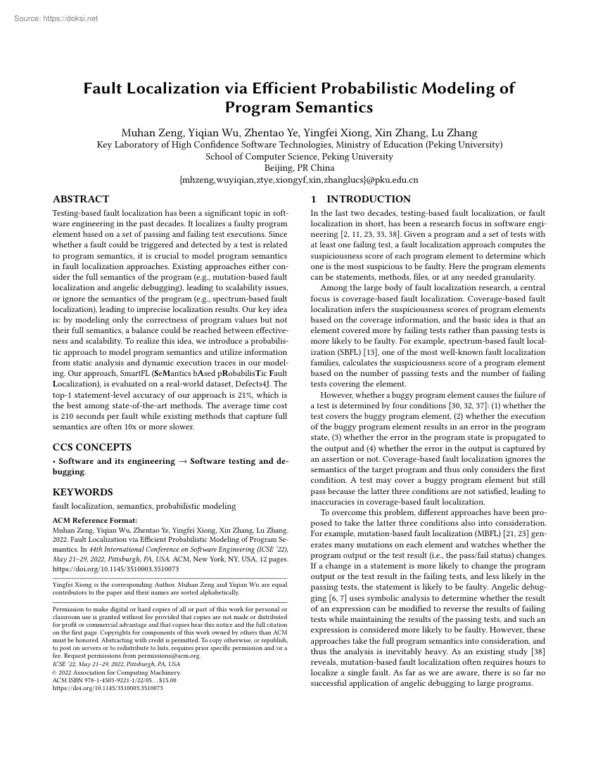
Section 2 motivates our approach with examples. Section 3 presents basic mathematical background about factor graphs. Section 4 describes our approach in detail, with an emphasis on how to build the probabilistic model. Section 5 shows the experiment results and answers the research questions. Section 6 discusses related research Section 7 concludes the paper. 2 OVERVIEW In this section, we motivate our approach using an example. Muhan Zeng, Yiqian Wu, Zhentao Ye, Yingfei Xiong, Xin Zhang, Lu Zhang 1 public class CondTest { 2 public static int foo ( int a ) { 3 if ( a <= 2) { // buggy , should be a < 2 4 a = a + 1; 5 } 6 return a ; 7 } 8 9 @Test 10 void pass () { 11 assertEquals (2 , foo (1) ) ; 12 } 13 14 @Test 15 void fail () { 16 assertEquals (2 , foo (2) ) ; 17 } 18 } Figure 1: A Motivating Example for Condition Modeling Motivating Example. Figure 1 (a) is a simple program for illustration purpose The buggy condition a <= 2 at line 3 replaced the correct condition a

< 2. There are two test cases to find the fault. For test pass, the fault does not influence the evaluation of the condition so the result is correct. However, in test fail, the fault misleads the test to the wrong branch and gets a wrong result. Here we assume statement-level fault localization, and a desirable approach should rank line 3 at the top. Coverage-based Approaches. We first demonstrate why coveragebased approaches such as SBFL fail to discover this bug Coveragebased approaches utilize code coverage information to calculate suspiciousness scores In SBFL approaches, the suspiciousness scores of an element � are calculated from four numbers: the number of passing tests covering �, the number of failing tests covering �, the total number of passing tests, and the total number of failing tests. However, in the above case, the coverage of passing tests and failing tests are completely identical, resulting in equal suspiciousness scores for every statement regardless of

specific SBFL formulas. As analyzed in the introduction, SBFL formulas cannot distinguish the suspicious degrees of different statements because coverage is only one out of the four conditions that lead to test failure. In test pass, though the faulty expression is covered, the resulted runtime state is still correct, and thus calculating suspiciousness with only coverage cannot distinguish each statement. Other Existing Approaches. To address the above challenge, many existing approaches try to analyze also the latter three conditions, i.e, whether the execution of a statement produces a faulty state, whether the faulty state is propagated to the output, and whether the test captures the fault in the state. However, to analyze the three conditions precisely, we need to consider the full semantics of the program, which is difficult to achieve efficiently. Here we analyze two families of approaches. A typical family is MBFL. MBFL mutates each statement to generate multiple mutants, and

check whether the output of each test execution [23] or the test result (i.e, the pass/fail status) [21] changes. In this case, mutating the statement at line 4 or the statement at line 6 has a high probability to fail test pass, while mutating the statement at line 3 has a much smaller probability to fail test pass. In this way, we know that the statement at line 3 has a weak Fault Localization via Efficient Probabilistic Modeling of Program Semantics correlation to the test result of pass and is more likely to be faulty. However, to obtain statistically significant information, we need to generate a number of mutants for each statement, and all tests need to be executed on each mutant, which takes a significant amount of time. In an existing empirical study [38], mutation-based fault localization requires hours to localize a single fault. Another example family is angelic debugging [6, 7]. Angelic debugging analyzes, for each expression, whether its result can be modified to

reverse the results of failing tests while maintaining the results of the passing tests. In this example, changing the result of expression a+1 at line 4 or the result of expression a at line 6 to any value different from 2 would fail test pass, and thus the two expressions are not considered to be buggy. However, such an analysis requires symbolic reasoning, which is known to be heavy and has limited scalability. So far there is no successful application of angelic debugging to large programs within our knowledge. Our Approach. Different from the above approaches, our approach takes a probabilistic view on fault localization Let us consider a sample space of all possible faults that the current program could potentially contain. Given the current test results as an observation, our approach estimates the probability of each program element being faulty. To efficiently estimate the probabilities, our approach builds a probabilistic model based on the probability that each statement

produces and propagates faulty values. Concretely, we introduce a set of Bernoulli random variables to represent whether a statement is correct, denoted by �� , where � is the line number of the statement. We also introduce another set of Bernoulli random variables to represent whether the output value of an expression execution is correct. In this example, we use ��,� (�� ,� ) to denote the value produced by the expression execution at line � in test pass (fail). Similarly, ��,2 and �� ,2 denotes the correctness of the test inputs and ��,6 and �� ,6 denotes the correctness of the test outputs. Since the input values of the tests are correct, we have the following probabilities. � (��,2 = 1) = � (�� ,2 = 1) = 1 Please note that since the Bernoulli random variables are binary, we also know � (��,2 = 0) = � (�� ,2 = 0) = 0. To ease presentation, we will only present one of the two probabilities. Since pass passes and fail fails,

we have the following probabilities. � (��,6 = 1) = 1 ∧ � (�� ,6 = 1) = 0 Now let us further consider the probabilities that the statements produce and propagate the faulty values. First, we notice that if the statement must be executed during the test execution, the statement itself is correct, and the input values are all correct, the result must be correct. Then we have the following conditional probability � (��,3 = 1 | � 3 = 1 ∧ ��,2 = 1) = 1 where � ∈ {�, � } � (��,6 = 1 | � 6 = 1 ∧ ��,4 = 1) = 1 Then, we notice that whether the statement at line 4 should be executed depends on the result of the expression at line 3. That is, if the expression produces the correct result, the executions of the statement at line 4 in the two tests are correct. Then we have the following conditional probability by considering both data and ICSE ’22, May 21–29, 2022, Pittsburgh, PA, USA control dependencies. � (��,4 = 1 | � 4 = 1 ∧

��,2 = 1 ∧ ��,3 = 1) = 1 where � ∈ {�, � } Next, we consider the case where faulty values may be produced or propagated. If an expression may produce a faulty result, any of the three following conditions must hold: the expression itself is wrong, the input of the expression is wrong, or the expression should not be executed. To simplify our probabilities model, we do not distinguish the three cases, and uniformly consider the probability that an expression returns a faulty value when some source is wrong. We notice that different types of operations behave differently. Some are very sensitive to the faults: when something goes wrong, the result is highly likely to be wrong. In our example, a+1 is such an operation. Some are insensitive to the faults: when something goes wrong, the result could still be correct. In our example, a <= 2 is such an operation. As a result, we give a high probability to the sensitive operations of returning a faulty value when something

is wrong and give a lower probability to the insensitive operations. As a result, we have the following probabilities. � (��,3 = 0 | � 3 = 0 ∨ ��,2 = 0) = 0.5 � (��,4 = 0 | � 4 = 0 ∨ ��,2 = 0 ∨ ��,3 = 0) = 0.99 where � ∈ {�, � } � (��,6 = 0 | � 6 = 0 ∨ ��,4 = 0) = 0.99 Based on the above probabilities, we build a factor graph [16] using these probabilities as references. Factor graph is a probabilistic graph modeling technique where constraints over the random variables could be easily added. Finally, we use a probabilistic inference algorithm named loopy belief propagation [25] to infer � (�� = 0) for each �. These probabilities reflect the suspiciousness In this example, we would successfully infer � (� 3 = 0) ≈ 0.707, � (� 4 = 0) ≈ 0.270, and � (� 6 = 0) ≈ 0223 � 3 has the highest probability to be faulty, i.e, successfully localizing the fault Challenges. While the basic idea is straightforward,

realizing this idea needs to address multiple challenges. The first challenge is modeling the effects of control statements. In Figure 2, the failing test goes through the else branch, leaving line 5 unexecuted, and thus fails the assertion. In this case, the value of a is incorrect, but the current modeling cannot relate this fault to the conditional expression at line 4 because a is not changed by any statement during the test execution. To overcome this problem, we need to model the effect of the unexecuted branch: the value of � could be faulty when the condition is faulty. We perform static analysis to obtain the variables changed by the unexecuted branch, i.e, a, and then add statement a=a after line 7 (denoted as line 7.1), ie, the end of the executed branch. Then following the same procedure, we would obtain the following conditional probability from the newly added statement: � (��,7.1 = 0 | � 71 = 0 ∨��,4 = 0 ∨��,2 = 0) = 099 where � ∈ {�, � } In

this way, the value of � and the value of the conditional expression are related. Finally, the suspiciousness score of the conditional expression at line 4 is assumed to be the maximum value of � (� 4 = 0) and � (� 7.1 = 0) The second challenge is scalability. This challenge comes from two aspects: (1) a project may contain many tests, and modeling ICSE ’22, May 21–29, 2022, Pittsburgh, PA, USA 1 public class Unexecuted { 2 public static int foo ( int a) { 3 int b = 0; 4 if (a < 10) // buggy , should be a <=10 5 a += 2; 6 else 7 b ++; 8 return a; 9 } 10 11 @Test 12 void pass () { 13 assertEquals (11 , foo (9) ) ; 14 } 15 16 @Test 17 void fail () { 18 assertEquals (12 , foo (10) ) ; 19 } 20 } Figure 2: An Example of Unexecuted Branch Muhan Zeng, Yiqian Wu, Zhentao Ye, Yingfei Xiong, Xin Zhang, Lu Zhang Figure 3: Approach Workflow. Multiple algorithms exist to infer the marginal distribution of the random variables. For example, loopy belief propagation [25]

is an efficient approximating algorithm to infer the marginal distributions. all of them may lead to a very large model, while many tests are unrelated to the current fault; (2) a test execution trace may be extremely long due to the existence of loops, while such long loops provide repeated information and modeling such a trace alone leads to a very large model. To address the first issue, we introduce a two-phase instrumentation, and use a coarse-grained instrumentation to filter out tests unrelated to the failing ones. To address the second issue, we introduce a loop compression algorithm to select typical iterations such that all control/data dependencies between statements and variables within any iteration are covered by at least one selected iteration. In this way, we model the main effects of the loop execution with a small number of iterations. We also introduce a compression method to compress the methods only covered by the passing tests as one node. The details can be

found in Sections 4.4 and 461 In this section, we first describe our approach in detail and then describe various optimizations we applied to scale it. Figure 3 shows the workflow of our approach. First, our approach instruments the subject program to generate execution traces of the test cases. Then, our approach applies static analysis on the whole program and dynamic analysis on the execution traces to extract control dependency and data dependency respectively. Next, our approach builds a probabilistic graphical model (i.e, a factor graph) based on this information that describes how the correctness of each program element affects each other. Finally, our approach adds results of the test cases as evidence to the model and performs marginal inference conditioning on them. Our approach ranks the statements based on their marginal probabilities and outputs this ranking. 3 4.1 BACKGROUND Before introducing our approach, we describe background information about factor graph [16],

which our probability model is based on. A factor graph is a bipartite graph representing the factorization of a probability distribution. The two parts of vertices are node vertices and factor vertices. Given a factor graph � = (�, �, �) consists of a node vertex set � = {� 1, � 2, . , �� }, a factor vertex set � = {�1, �2, . , �� } and an edge set � Each node �� ∈ � represents a random variable in the distribution. Each factor � � ∈ � represents a multivariate function, mapping from some of the random variables to a real value representing the relative likelihood of the event. If there is an edge from �� to � � , �� is an input variable of � � . Let � � ⊆ � be the set of the input variables of � � . The production of all factors represents the probabilistic weight. Therefore, the joint probability distribution can be defined as Î� �=1 � � (� � ) Î� � (� 1, � 2, . , �� ) = Í �

1 ,� 2 ,.,�� �=1 � � (� � ) Notice that the denominator representing the total probabilistic weight from the entire sample space is used to normalize the probability. 4 OUR APPROACH Instrumentation Our approach instruments test runs at the bytecode level and collects traces that are further used in dependency analysis. Concretely, our trace includes a sequence of instruction executions, where each instruction execution includes the ID of the instruction, the type of the instruction, the values read/written by this instruction, and the change to the program counter. To facilitate understanding, we will describe our approach at the Java source code level, and use “statement” and “instruction” interchangeably. Yet the readers should be aware that the collected traces are at the level of bytecode. 4.2 Dependency Analysis Modeling dynamic data dependency can easily be done by utilizing the information from collected traces. For any read operation on a memory

location, the most recent write and its corresponding instruction can be resolved by sequentially iterating instructions in the trace while keeping track of all memory writes. This information is used in building the probabilistic graph described in Section 4.3 Besides data dependencies, we also need to consider control dependencies to precisely model how errors are introduced and propagated. Unlike modeling data dependencies, we need to consider information from the whole program rather than only from Fault Localization via Efficient Probabilistic Modeling of Program Semantics ICSE ’22, May 21–29, 2022, Pittsburgh, PA, USA 1 public int foo (.) { 2 if ( condition ) 3 return a; 4 . 5 return b; 6 } Figure 4: Example Program Demonstrating Control Dependencies. traces. To decide whether a branching statement controls another statement in execution, one needs to investigate whether the statement would still be executed if the branching statement turns to a different branch other

than the one taken in the execution. This can only be achieved with the information of program fragments enclosed in the unexecuted branch. Consider the program in Figure 4 Suppose in a concrete run, the program takes the false branch, and thus the trace is if(false) . return b The trace does not include the information of the true branch and it remains unclear whether line 5 would be executed if the true branch was taken. However, by investigating the program, we know that the dependency holds as the method will return at line 3 if the branching statement takes the true branch. As a result, the branching statement controls all other statements in the method, as its branching status affects all other statements being executed or not. To precisely model control dependencies, we apply a static analysis [8] that calculates dominance relations [3] between statements on control flow graphs. Intuitively, a control statement controls all its subsequent statements in its control flow graph

until it reaches statements that post-dominate it. 4.3 Building the Probabilistic Graph After dependency analysis, our approach builds a factor graph (described in Section 3) that models how errors are introduced and propagated based on dependency information and program semantics. In the graph, a node denotes a random variable that represents the correctness of a statement or a run-time variable’s value; edges are added based on control and data dependencies; factors describe how likely errors can be introduced or propagated in a certain way. An example factor graph is shown in Figure 5 We next describe each component in detail. Nodes. A node is a Bernoulli random variable that represents the correctness of a run-time value or a statement. The former is called a value-node, and the latter is called a statement-node. Our approach adds a value-node to the graph whenever an assignment occurs on a variable or a field in the trace. Thus a variable/field corresponds to multiple nodes

in the graph, each of which corresponds to a value it holds during executions. As for statements, we create only one statement-node for each statement in the program as a statement’s correctness should be consistent among all test executions. Thus, sub-graphs constructed from different test cases are connected through statement-nodes. Edges. Edges are added based on the control and data dependencies In a factor graph, nodes are not directly connected, and an edge always connects a node to a factor. There are two types of factors in our model: semantics-factors and evidence-factors. Figure 5: Generated factor graph for Figure 1. Semantics-factors and evidence-factors add program semantics and observation evidence to our model respectively, which we will discuss later. For a node whose correctness is known (e.g from the test oracle), we introduce an evidence-edge to link it with a corresponding evidence-factor. For each statement, we introduce a semantics-factor and corresponding

edges to describe how errors can be introduced by it or propagated through it. Concretely, the following nodes are connected to the semantics-factor: (1) The statement-node itself. (2) A value-node that represents the value that is written by the statement. (3) Value-nodes that represent values that are read in the statement. (4) Value-nodes that represent the condition values that control the current statement. The corresponding edges that connect to these nodes are called: statement-edge, define-edge, use-edge, and control-edge, respectively. These edges together link a value-node denoting the result of the statement ((2)) with its possible immediate sources of errors ((1)(3)(4)). Factors. As described in Section 3, each factor represents a multivariate function In our model, the function of a semantics-factor evaluates how likely a value can become erroneous after executing a statement. The main idea is that if any of the following: (1) The current statement (2) All values it uses

(3) All condition values that controls it is erroneous, then there is a possibility that the value it defines is erroneous. We refer to all the three former elements as “sources”, and the last one as “result” in the rest of this section. Table 1 shows the function of semantics-factors. The column “Sources” indicates whether all the sources are correct, while the ICSE ’22, May 21–29, 2022, Pittsburgh, PA, USA Muhan Zeng, Yiqian Wu, Zhentao Ye, Yingfei Xiong, Xin Zhang, Lu Zhang Table 1: The truth table of a semantics-factor. Sources Result 1 1 0 0 1 0 1 0 Factor Value Insensitive Sensitive 1 0 0.5 0.5 1 0 0.01 0.99 column “Result” indicates whether the result is correct. The “Factor Value” column indicates the likelihood of different correctness states of sources and the result. Note the factor values cannot be directly interpreted as probabilities, but as a way to compare the likelihood between different states of sources and the result. Further, we

observe that statements whose operators are “<”, “>”, “==”, “!=” or “%” are less sensitive to the correctness of the sources than other operators (e.g “+” , “×”) For example, when � contains an incorrect value, there is a higher chance for � > 0 to produce a correct value than � + 1, as the prior has a much smaller value domain {True, False}. Following this intuition, we divide the “Factor” column into “Insensitive” and “Sensitive” for these two types of statements. We now explain the meaning of each row in the table. The first two rows mean that when all the sources are correct, the statement should always produce a correct result. The last two rows mean that when the sources are not fully correct, there is still a chance for the result to be correct. For insensitive statements, such a chance is moderate (0.5), which is the same as the chance for the result to be incorrect. While for sensitive statements, such a chance is very

low (0.01), and the chance for the result to be incorrect is very high (0.99) We refer to parameters 05, 001, and 099 as moderate, very low, and very high factor values in Section 5, and the impact of different parameter values is further discussed in RQ3. Finally, we can infer the correctness of some program elements from test inputs and test assertions. Most notably, we have the followings: (1) Test inputs should be correct. (2) The Boolean value produced by passing assertions should be correct. (3) The Boolean value produced by failing assertions should be incorrect. We add these information to our model as follows: for each evidence (� = �), an evidence-factor linking to the corresponding program element is added to the graph, with the factor function defined as follows: � (� = �) = 1 and � (� ≠ �) = 0. 4.4 Capturing Semantic Effect of Unexecuted Statements So far, we have introduced how to model the data dependencies and control dependencies between statements

that are executed in test cases. However, this information is not enough to locate faults precisely because an error can be introduced if necessary statements are not executed. Consider the example in Figure 2 again The assertion on line 18 fails because the statement on line 5 is not executed, which is further caused by the incorrect branching statement on line 4. However, one cannot capture this connection by only reasoning about control dependencies and data dependencies recovered from the trace. To model this information precisely, one needs to also reason about data dependencies and control dependencies between executed code and unexecuted code. However, a full-fledged static analysis that considers all possible behaviors of the program would be too expensive. Instead, we take a lightweight approach that abstracts the effect of unexecuted code by transforming the original program. Briefly, for a condition �, let S be the set of all variables defined by the statements controlled

by �. For each variable � in �, the transformation adds a complementary statement � = � at the end of each branch. The complementary statement is regarded as the branching statement in the result, as the incorrectness of � = � means the program has taken the wrong branch. For simplicity, we only consider variables on the stack in our implementation. Such a transformation does not change the program’s semantics but allows our control dependency analysis and data dependency analysis to abstract the effect of unexecuted code automatically. 4.5 Getting the Final Result The factor graph that is built using the above steps defines a joint distribution of the correctness of all program elements. We now can perform a marginal inference on the graph, which produces the probability of a program element being incorrect. This in turn is used to produce the final ranking of fault localization. We implement the inference using an efficient iterative algorithm called loopy belief

propagation [25]. Finally, we perform dynamic slicing to filter elements irrelevant to the fault. 4.6 Scaling Our Approach Instrumenting program runs can produce enormous execution traces. These can lead to gigantic factor graphs which cannot even be stored in physical memory, let alone performing inference. To address this challenge, we apply several techniques to reduce the trace sizes within and across test cases. 4.61 Reducing Sizes of Traces We apply two techniques to reduce the size of a given trace: compressing loops, and selectively instrumenting methods. As pointed out in Section 2, heavy loops may lead to long traces, resulting in a very large model. In addition, it also contains repeated code patterns, which provides very little information to our probabilistic model. To reduce the trace caused by the loops, we would like to select a key subsequence of the trace containing some of the iterations. Here we define a subsequence as a key subsequence if all control/data

dependencies between statements and variables within any iteration are covered by at least an iteration in the subsequence. In this way, we can model the main effect of the loop while significantly reducing its size. To select the key subsequence, we check each pair of adjacent iterations. If the sequences of statements executed in the two iterations are identical, we only keep the first iteration in the final trace. As for nested loops, we first compress the inner loops and then compress the outer loops. As a result, for any sequence of statements executed, at least an iteration is kept to represent the Fault Localization via Efficient Probabilistic Modeling of Program Semantics sequence. Accordingly, all control/data dependencies are kept with respect to the key subsequence. Second, we observe that parts of the passing traces can be summarized into atomic statements. The key insight is that the incorrect statements that are responsible for the failure must be covered by at least

one of the failing test cases. As a result, for a sequence of statements that are only covered in passing test cases, we only care about the dependencies between them and other statements but not the dependencies between statements inside the sequence, because none of them can be the faulty statement our approach is trying to locate. This sequence in turn can be treated as one atomic statement We perform such compression at method levels as statements inside them usually have limited dependencies with statements outside them. For example, when a method does not access the heap, it can be summarized as a statement that calculates its return value based on the parameters. Concretely, we also consider field access of the callee object when the method is non-static, as setters and getters are very common practices in Java that involve field access. 4.62 Selecting Test Cases While our techniques are effective in reducing trace sizes, some of the traces can be still too large to be included.

Therefore, we introduce several techniques to select a subset of test cases whose information will be included in our modeling. First, we observe that while all failing test cases usually carry useful information about faults, not all passing test cases are useful. In particular, if a passing test has a completely different coverage compared to failing tests, it carries no information for localization as it does not cover any suspicious location. Similarly, if a passing test case covers a very different set of methods compared with the failing test cases, it is unlikely it is useful in locating the faults. To realize this idea, we first run a coarse-grained instrumentation to get method-level coverage. The tests are ranked by the number of commonly covered methods with failing tests. Except for the top 50 tests, the remaining tests are excluded from fine-grained instrumentation, which is often costly because of heavy I/O. Second, due to practical concerns, we exclude very long traces

and some traces when the probabilistic graph becomes too large. To handle the former case, we set a hard limit on the size of any given trace and discard traces whose size has reached this limit. To handle the second case, we set a limit on the size of the probabilistic graph under construction. More concretely, when constructing a graph, we consider all failing test cases. As for passing test cases, we sort their traces by the size in ascending order and add their information one-by-one to the graph until the graph size reaches the limit. 5 EVALUATION 5.1 Research Questions • RQ1: Effectiveness of SmartFL. How effective is SmartFL compared to other techniques? • RQ2: Efficiency of SmartFL. What is the time cost of SmartFL compared to other techniques? • RQ3: Influence of Different Factor Values. To what extent do moderate, very low, and very high factor values in both sensitive and insensitive statements affect the results? ICSE ’22, May 21–29, 2022, Pittsburgh, PA, USA

Table 2: Projects from Defects4j dataset, version 1.01 Project Faults LoC Apache Commons Math Apache Commons Lang Joda-Time JFreeChart Total 106 64 26 26 222 103.9k 49.9k 105.2k 132.2k 91.7k ’Faults’ denotes the number of defective versions of the project, ’LoC’ denotes the average lines of code of each project. Bold denotes the abbreviation for the project. • RQ4: Effectiveness of Different Components. What is the contribution of each component to the overall effectiveness? • RQ5: Combining with other Techniques. Can SmartFL improve the effectiveness of combination methods? 5.2 Benchmark and Measurements We take the projects from Defects4j [15] version 1.0 as our benchmark, so as to compare with the results of other approaches in existing studies [26, 38]. We exclude the Closure project because it contains many advanced language features as a compiler implementation, which our current implementation does not support. We also exclude bugs “Lang-2” and

“Time-21” because they are no longer reproducible due to deprecation. As a result, our dataset includes four projects, 222 faults, as shown in Table 2. Our evaluating metric is top-k where � is 1, 3, 5, or 10. Top-k counts the number of faults that are successfully located within the top k entries of the ranked suspicious candidate list. An existing study [24] suggested that developers would only check a few entries in the ranked list, which is consistent with the top-k metric. We follow the measurement rules provided in a previous study [38]. Regarding the granularity of fault localization, we choose both statement-level and method-level granularity, the two most frequently used levels. As for method-level evaluation, we calculate the suspicious score of a method as the maximum suspicious score of its statements, e.g the method’s ranking is equal to its highestranking statement 5.3 Experiment Setup 5.31 Implementation We have implemented our approach for Java using the

instrumentation framework Javassist1 . The instrumentation causes JVM crashes on some of the subjects in our experiments, and we deem that our approach fails to localize the fault for these subjects. As described in Section 4.6, we select up to 50 test methods for tracing and limit the maximum number of lines to be less than 1.2 million for each trace. Upon building the graph, we limit the maximum number of lines to be less than 1 million for all compressed traces. Please note that this selection only applies to our approach but not any other baseline approach. Our implementation may still 1 https://github.com/jboss-javassist/javassist ICSE ’22, May 21–29, 2022, Pittsburgh, PA, USA run out of memory after the selection on some subjects, and we treat these cases as failures of our approach to localize the fault. Our current implementation does not support some advanced Java features such as reflection and may miss data and control dependencies introduced by these features. This

incomplete modeling may reduce the performance, yet our approach still shows significant advantages over existing approaches despite this implementation issue. Muhan Zeng, Yiqian Wu, Zhentao Ye, Yingfei Xiong, Xin Zhang, Lu Zhang Table 3: Statement-level Performance Project Technique Top-1 Top-3 Top-5 Top-10 Total Ochiai DStar Metallaxis MUSE SmartFL 11(5%) 12(5%) 21(9%) 17(8%) 47(21%) 64(29%) 65(29%) 69(31%) 35(15%) 80(36%) 86(39%) 86(39%) 89(40%) 45(20%) 97(44%) 118(53%) 117(53%) 111(50%) 50(23%) 118(53%) 5.32 RQ1: Effectiveness of SmartFL To test the effectiveness of SmartFL, we compare the result of SmartFL with SBFL, representing coverage-based approaches, and MBFL, representing the approaches modeling semantics. We do not compare with angelic debugging because there is no implementation scalable to large programs as far as we know. According to existing research [38], we select Ochiai [2] and DStar [33] from SBFL, Metallaxis [23] and MUSE [21] from MBFL for

comparison, and the performance data of these approaches are obtained from an existing study [38]. 5.33 RQ2: Efficiency of SmartFL We compare the run-time cost of SmartFL with the four baseline approaches described in RQ1. As Figure 3 shows, SmartFL consists of two steps: (a) tracing and (b) modeling (including probabilistic inference). In the tracing step, tracing each test can be run in parallel except project Time because the tests of Time do not support parallel execution. As a result, we run tests in parallel with 16 threads for the other three projects and run tests with a single thread for Time. In the modeling step, we run modeling and probabilistic inference in a single thread. 5.34 RQ3: Influence of Different Factor Values We assign 05-05 to the factor values of insensitive operations and 0.01-099 to those of sensitive operations in our default approach. In this RQ we evaluate the performance of other possible values. We evaluate 9 pairs of factor values for insensitive

operations: 0.1 − 09, 02 − 08, , 09 − 0.1, and 4 pairs of those for sensitive operations: 0001−0999, 001− 0.99, 005 − 095, 01 − 09 This experiment is taken only on project Lang rather than the whole dataset to save time. 5.35 RQ4: Effectiveness of Different Components We design two ablation studies to evaluate the effectiveness of two components. In the first study, we discard the modeling of unexecuted statements described in Section 4.4 and compare the results on all 222 cases In the second study, we discard loop compression described in Section 4.61 and compare the results and time cost on the modeling step with the original version, on the cases that do not trigger the limit of total trace lines when discarding loop compression. The selection ensures all added traces are identical in both versions. 5.36 RQ5: Combining with other Techniques CombineFL [38] is the state-of-the-art fault localization technique on statement-level. We combine SmartFL with other methods

under the framework of CombineFL on all 222 cases. CombineFL requires a suspiciousness score for each standalone technique to perform learning. In SmartFL, the suspiciousness score of an ��ℎ − ������ statement is defined as follow: � −� +1 �������������� (�) = � Where � is the number of all suspicious candidates. Table 4: Sign Test Result Method Positive Negative P-value vs. Ochiai vs. DStar vs. Metallaxis vs. Muse 87 88 80 100 58 59 64 36 0.01974 0.02061 0.2112 3.72e-08 Table 5: Method-level Performance Project Technique Top-1 Top-3 Top-5 Top-10 Total Ochiai DStar Metallaxis MUSE SmartFL 73(33%) 75(34%) 70(31%) 44(20%) 96(43%) 138(62%) 140(63%) 129(58%) 71(32%) 136(61%) 156(70%) 155(70%) 149(67%) 83(37%) 155(70%) 176(79%) 177(80%) 166(75%) 91(41%) 176(79%) 5.4 Experiment Results 5.41 RQ1: Effectiveness of SmartFL Table 3 shows the numbers and percentages of faults localized by different approaches at

statementlevel. Here, we describe a fault is successfully localized by an approach if the actual fault position can be found in the top k program elements returned by the approach. We display the results with different values of k in the top-k metric. The best results under each category are in bold fonts. On all the 222 faults, SmartFL performs best among all values of k. At top-1, 3, and 5, SmartFL improves 114%, 16%, and 9% over the second-best approach, respectively. At top-10, SmartFL has the same performance as Ochiai. We also perform a sign test on each pair of techniques considering faults where at least one technique has a top-10 result on it, and the result is shown in Table 4. We confine the test to these faults because a difference between rank 100 and 1000 would not make a great difference in actual use cases. The result implies that our method significantly outperforms Ochiai, DStar, and Muse, while still having more positive than negative cases compared with Metallaxis.

Still, the negative cases in the sign test show that our method could be complementary to others, which is further discussed in RQ5. Table 5 shows the performance of each approach at method level. SmartFL performs better than Metallaxis and MUSE using all top-k metrics. SmartFL has an advantage over Ochiai and Dstar at top-1 and roughly the same effect as they have at top-3,5 and 10. Fault Localization via Efficient Probabilistic Modeling of Program Semantics ICSE ’22, May 21–29, 2022, Pittsburgh, PA, USA Table 6: Average Time Consumption of each Technique (in seconds, to 2 digits of precision) Technique Average Lang Math Chart Time CPU Ochiai DStar Metallaxis MUSE 64 64 3500 3500 26 26 270 270 86 86 3000 3000 44 44 5400 5400 85 85 12000 12000 2.40GHz SmartFL 210 51 140 280 830 2.10GHz Table 7: Different Moderate Factor Values for Insensitive Operations Table 8: Different Very low/Very high Factor Values for Sensitive Operations Value Total Top-1

Top-3 Top-5 Top-10 0.001-0999 139 22(34%) 34(53%) 37(58%) 46(72%) 0.01-099 140 21(33%) 34(53%) 39(61%) 46(72%) 0.05-095 144 21(33%) 35(55%) 41(64%) 47(73%) 0.1-09 144 21(33%) 33(52%) 42(66%) 48(75%) Table 9: Effect of Modeling Unexecuted Statements. Technique Top-1 Top-3 Top-5 Top-10 Origin w/o Unexecuted 47 48 80 80 97 95 118 118 Value Total Top-1 Top-3 Top-5 Top-10 0.1-09 133 19(30%) 32(50%) 37(58%) 45(70%) 0.2-08 138 21(33%) 35(55%) 39(61%) 43(67%) 0.3-07 139 21(33%) 35(55%) 39(61%) 44(69%) 0.4-06 141 21(33%) 35(55%) 39(61%) 46(72%) 0.5-05 140 21(33%) 34(53%) 39(61%) 46(72%) Technique Time Top-1 Top-3 Top-5 Top-10 0.6-04 141 21(33%) 34(53%) 39(61%) 47(73%) 0.7-03 142 22(34%) 34(53%) 38(59%) 48(75%) Origin w/o Compression 30s 49s 33 31 50 49 57 56 65 64 0.8-02 139 22(33%) 32(50%) 39(61%) 46(72%) 0.9-01 138 22(33%) 32(50%) 38(59%) 46(72%) SmartFL focuses on statement-level

fault localization and SmartFL performs better than all other techniques on statement-level. At method-level, SmartFL still significantly outperforms others in terms of Top-1 accuracy. The above results demonstrate the effectiveness of SmartFL 5.42 Efficiency of SmartFL Table 6 shows the time costs of all techniques. The performance data of the baselines are obtained from an existing study by Zou et al. [38] The execution time is not directly comparable because the two experiments are on different hardware platforms. However, we cannot reproduce the experiments by Zou et al [38] because the implementation only supports an old version of Defects4J, which is no longer available. Nevertheless, the hardware platforms for the two sets of experiments have CPUs with similar lock speed2 , and thus significant time difference still matters. As mentioned in Section 5.3, we run tests with a single thread on benchmark Time so the time cost for Time is much longer than those of other projects. The

average time of SmartFL is 210 seconds, which is an order of magnitude smaller than MBFL methods. The result shows SmartFL models the semantics of the program in an efficient way. 2 Intel Xeon E5-2640 v4@2.40GHz-12 cores ([38]) vs Intel Xeon Gold 6230@210GHz-20 cores (ours) Table 10: Effect of Loop Compression (on 93 selected cases). 5.43 RQ3: Influence of Different Factor Values We re-run our approach on project Lang with different factor parameters (moderate, very low, and very high) for both sensitive and insensitive statements. The result is shown in Table 7 and Table 8 In the first column, the former number denotes the factor value of getting the correct result when receiving wrong sources and the latter number denotes the factor value of getting the wrong result. We can see that the choice of parameters has only a small impact on the results. This suggests that our model is robust with respect to different parameters, and could still work without fine-tuning. 5.44 RQ4:

Effectiveness of Different Components We perform several ablation studies to evaluate the effect of different components of our approach. Table 9 shows the effect of modeling unexecuted statements. Without considering the effect of unexecuted statements, the top-1 and top-5 results receive a small change. In general, the effect of modeling unexecuted statements is not significant. However, we notice that the results on 63 out of 222 cases changed, and particularly, “Lang 53” and “Math 79” failed when unexecuted statements are not modeled. The two newly introduced failures suggest some Defects4J cases can be successfully localized by SmartFL only with the help of modeling unexecuted statements. Following the rules described in Section 5.35, we select 93 cases that do not exceed the limit of total trace lines in the benchmark. Table 10 shows that the default approach performs slightly better, which suggests removing redundant sequences from traces could effectively reduce

execution time while preserving effectiveness. ICSE ’22, May 21–29, 2022, Pittsburgh, PA, USA Muhan Zeng, Yiqian Wu, Zhentao Ye, Yingfei Xiong, Xin Zhang, Lu Zhang Table 11: Integrating SmartFL with CombineFL Technique Top-1 Top-3 Top-5 Top-10 CombineFL Level-2 32(14%) 93(42%) 116(52%) 144(64%) SmartFL with Level-2 58(26%) 102(47%) 124(56%) 144(64%) CombineFL Level-4 45(20%) 95(43%) 121(55%) 143(64%) SmartFL with Level-4 53(24%) 97(44%) 127(57%) 149(67%) is also inspired by their work, but there are multiple fundamental differences: (1) To easily integrate the developers’ feedback, their approach uses two-level reasoning, first calculating the faulty probabilities of the runtime values and then calculating the faulty probabilities of the statement. As a result, different test executions are isolated and thus their approach cannot support fault localization from multiple tests. (2) Their approach does not consider the effect of the unexecuted

branches. (3) Their approach does not select nor compress test executions. Difference (1) is essential in our problem, as the passing tests provide critical information for fault localization and cannot be ignored. In the example in 1, without the passing tests, we cannot localize correctly. Differences (2) and (3) are evaluated in RQ4, which indicates that removing them leads to a performance drop. 5.45 RQ5: Combining with other Techniques CombineFL is a technique for combining different fault localization methods CombineFL has four levels, each consists of standalone techniques with time cost under a certain level. Level-2 contains only lightweight methods that require minutes to run, including history-based, stack trace-based, IR-based, slicing, and SBFL methods. Compared with level-2, level-4 further includes predicates switching and MBFL, which usually requires more than an hour to localize the faults. By excluding heavy-weight approaches and including SmartFL in CombineFL, the

time cost is greatly reduced as SmartFL only requires minutes to localize one fault. We also combine SmartFL with Level-4 CombineFL to show our full potential. The result is shown in Table 11. The top-1 accuracy raises to 58 (26%) by replacing MBFL methods with SmartFL, while combining with Level-4 results in better Top-10 accuracy. We notice that combining more techniques to SmartFL with CombineFL Level-2 may drop Top1 accuracy. The reason could be that SmartFL’s result is correlated to MBFL’s result but still has a difference. The result also shows a new learning method may better combine SmartFL and MBFL, and calls for further research. As mentioned before, the main type of coverage-based fault localization is SBFL approaches, which calculates the suspicious scores of program elements based on the numbers of pass/fail tests covering the element using different formulas [1, 12, 22]. As mentioned, coverage is only one of the four conditions for a test to fail on a fault, and thus

the coverage-based approaches do not consider the latter three conditions. To overcome this problem, some existing approaches combine SBFL with program slicing [14, 20, 29], in the sense that only the statements in the slice can produce and propagate the faults. For example, Mao et al [20] proposed SSFL (slice-based statistical fault localization). By calculating the suspiciousness score on an approximate dynamic backward slice, SSFL significantly boosts all 16 formulas of SBFL. However, slicing only reveals the possibility but not the probability that a program element produces or propagates fault, and thus is a very inaccurate modeling of semantics. 6 6.3 RELATED WORK Fault localization has been intensively studied during the past decades. Here we leave a full summary of fault localization to respectively surveys [4, 28, 34] and empirical studies [38], and discuss only the most related work. 6.1 Probabilistic Approaches Fault localization is inherently a probabilistic analysis

process, and many existing approaches resort to probabilistic modeling. Similar to our approach, these modeling approaches also treat the sample space as all possible faults or all possible fault locations and try to identify the element that has the highest conditional probability to be faulty based on the observed test results. Different from our approach that extract the probabilities from the semantics of the program, most probabilistic approaches either consider only the coverage and do not model the semantics of the program [10, 27], or learn the probabilities from test executions [5, 9]. The only exception is Xu et al. [35]’s approach This approach solves a different problem, namely interactive fault localization: how to support the developer when he faces one failing test. Similar to our approach, their approach also uses probabilistic modeling and introduces Bernoulli probabilistic variables to represent whether the runtime values and statements are faulty or not. Our

approach 6.2 Spectrum-based Fault Localization Approaches Modeling Semantics As we have carefully discussed in Sections 1 and 2, MBFL [21, 23] and angelic debugging [6, 7] are the two main families that model semantics for fault localization, but both have scalability issues due to their precise modeling of the semantics. Our evaluation also shows that our approach is about 10X faster than MBFL and is much more effective. 6.4 Combination Approaches Multiple approaches try to combine existing approaches or different information sources. Xuan and Monperrus [36] proposed a learning-to-rank approach to integrate the suspiciousness scores of 25 existing SBFL formulae. Zou et al [38] further extended this approach to integrate the suspiciousness scores produced by different families of fault localization families. Our approach could also be integrated using these approaches. As our evaluation shows, our approach could significantly boost the performance of the combined approaches.

Other approaches try to use machine learning techniques to combine different information sources. For example, Sohn and Yoo [31] use the learning-to-rank technique to combine the suspiciousness scores of existing SBFL formulae, code complexity metrics, and code history metrics; Li et al. [18] use neural network to combine Fault Localization via Efficient Probabilistic Modeling of Program Semantics suspiciousness scores of SBFL and MBFL, code complexity metrics, and text similarity metrics; Küçük et al. [17] use causal inference techniques and machine learning to integrate predicate outcomes and runtime values; Lou et al. [19] use neural network to embed both the syntax of the program and the coverage information. However, none of these approaches are able to integrate the semantic information, which is the focus of this paper. 7 CONCLUSION This paper proposes a novel fault-localization method based on probabilistic graph model. Specifically, we utilize semantic information

of different statements, while combining both dynamic and static information into our model. We conduct an experiment on a real-world dataset, Defects4J. Our technique is evaluated to be complementary to existing techniques as it could further improve state-of-the-art by combining with existing techniques. To facilitate research, our tool and the fault localization data are available at https://github.com/toledosakasa/SMARTFL ACKNOWLEDGMENTS We acknowledge Jingjing Liang and Daming Zou for sharing their experiment data [38]. This work is sponsored by National Natural Science Foundation of China under Grant No. 61922003 and No 62172017. REFERENCES [1] Rui Abreu, Peter Zoeteweij, and Arjan JC Van Gemund. 2006 An evaluation of similarity coefficients for software fault localization. In 2006 12th Pacific Rim International Symposium on Dependable Computing (PRDC’06). IEEE, 39–46 [2] Rui Abreu, Peter Zoeteweij, and Arjan JC Van Gemund. 2007 On the accuracy of spectrum-based fault

localization. In Testing: Academic and industrial conference practice and research techniques-MUTATION (TAICPART-MUTATION 2007). IEEE, 89–98. [3] Alfred V. Aho, Ravi Sethi, and Jeffrey D Ullman 1986 Compilers: Principles, Techniques, and Tools. Addison-Wesley https://wwwworldcatorg/oclc/12285707 [4] Mohammad Amin Alipour. 2012 Automated fault localization techniques: a survey. Oregon State University 54, 3 (2012) [5] George K. Baah, Andy Podgurski, and Mary Jean Harrold 2010 The Probabilistic Program Dependence Graph and Its Application to Fault Diagnosis. IEEE Trans Software Eng. 36, 4 (2010), 528–545 https://doiorg/101109/TSE200987 [6] Satish Chandra, Emina Torlak, Shaon Barman, and Rastislav Bodik. 2011 Angelic debugging In Proceedings of the 33rd International Conference on Software Engineering. 121–130 [7] Maria Christakis, Matthias Heizmann, Muhammad Numair Mansur, Christian Schilling, and Valentin Wüstholz. 2019 Semantic Fault Localization and Suspiciousness Ranking In

Tools and Algorithms for the Construction and Analysis of Systems - 25th International Conference, TACAS 2019, Held as Part of the European Joint Conferences on Theory and Practice of Software, ETAPS 2019, Prague, Czech Republic, April 6-11, 2019, Proceedings, Part I (Lecture Notes in Computer Science, Vol. 11427), Tomás Vojnar and Lijun Zhang (Eds) Springer, 226–243 https://doi.org/101007/978-3-030-17462-0 13 [8] Keith D Cooper, Timothy J Harvey, and Ken Kennedy. 2001 A simple, fast dominance algorithm. Software Practice & Experience 4, 1-10 (2001), 1–8 [9] Laura Dietz, Valentin Dallmeier, Andreas Zeller, and Tobias Scheffer. 2009 Localizing Bugs in Program Executions with Graphical Models In Advances in Neural Information Processing Systems 22: 23rd Annual Conference on Neural Information Processing Systems 2009. Proceedings of a meeting held 7-10 December 2009, Vancouver, British Columbia, Canada, Yoshua Bengio, Dale Schuurmans, John D Lafferty, Christopher K I Williams,

and Aron Culotta (Eds) Curran Associates, Inc., 468–476 https://proceedingsneuripscc/paper/2009/ hash/f64eac11f2cd8f0efa196f8ad173178e-Abstract.html [10] Alberto González-Sanchez, Rui Abreu, Hans-Gerhard Groß, and Arjan J. C van Gemund. 2011 Spectrum-Based Sequential Diagnosis In Proceedings of the Twenty-Fifth AAAI Conference on Artificial Intelligence, AAAI 2011, San Francisco, California, USA, August 7-11, 2011, Wolfram Burgard and Dan Roth (Eds.) AAAI Press. http://wwwaaaiorg/ocs/indexphp/AAAI/AAAI11/paper/view/3565 ICSE ’22, May 21–29, 2022, Pittsburgh, PA, USA [11] Jiajun Jiang, Ran Wang, Yingfei Xiong, Xiangping Chen, and Lu Zhang. 2019 Combining spectrum-based fault localization and statistical debugging: an empirical study. In 2019 34th IEEE/ACM International Conference on Automated Software Engineering (ASE). IEEE, 502–514 [12] James A Jones and Mary Jean Harrold. 2005 Empirical evaluation of the tarantula automatic fault-localization technique In Proceedings of

the 20th IEEE/ACM international Conference on Automated software engineering. 273–282 [13] James A Jones, Mary Jean Harrold, and John Stasko. 2002 Visualization of test information to assist fault localization. In Proceedings of the 24th International Conference on Software Engineering. ICSE 2002 IEEE, 467–477 [14] Xiaolin Ju, Shujuan Jiang, Xiang Chen, Xingya Wang, Yanmei Zhang, and Heling Cao. 2014 HSFal: Effective fault localization using hybrid spectrum of full slices and execution slices. Journal of Systems and Software 90 (2014), 3–17 [15] René Just, Darioush Jalali, and Michael D Ernst. 2014 Defects4J: A database of existing faults to enable controlled testing studies for Java programs In Proceedings of the 2014 International Symposium on Software Testing and Analysis. 437–440 [16] Frank R Kschischang, Brendan J Frey, and H-A Loeliger. 2001 Factor graphs and the sum-product algorithm. IEEE Transactions on information theory 47, 2 (2001), 498–519. [17] Yigit Küçük,

Tim A. D Henderson, and Andy Podgurski 2021 Improving Fault Localization by Integrating Value and Predicate Based Causal Inference Techniques. In 43rd IEEE/ACM International Conference on Software Engineering, ICSE 2021, Madrid, Spain, 22-30 May 2021. IEEE, 649–660 https://doiorg/101109/ ICSE43902.202100066 [18] Xia Li, Wei Li, Yuqun Zhang, and Lingming Zhang. 2019 DeepFL: integrating multiple fault diagnosis dimensions for deep fault localization. In Proceedings of the 28th ACM SIGSOFT International Symposium on Software Testing and Analysis, ISSTA 2019, Beijing, China, July 15-19, 2019, Dongmei Zhang and Anders Møller (Eds.) ACM, 169–180 https://doiorg/101145/32938823330574 [19] Yiling Lou, Qihao Zhu, Jinhao Dong, Xia Li, Zeyu Sun, Dan Hao, Lu Zhang, and Lingming Zhang. 2021 Boosting coverage-based fault localization via graphbased representation learning In ESEC/FSE ’21: 29th ACM Joint European Software Engineering Conference and Symposium on the Foundations of Software

Engineering, Athens, Greece, August 23-28, 2021, Diomidis Spinellis, Georgios Gousios, Marsha Chechik, and Massimiliano Di Penta (Eds.) ACM, 664–676 https://doiorg/10 1145/3468264.3468580 [20] Xiaoguang Mao, Yan Lei, Ziying Dai, Yuhua Qi, and Chengsong Wang. 2014 Slice-based statistical fault localization. Journal of Systems and Software 89 (2014), 51–62. [21] Seokhyeon Moon, Yunho Kim, Moonzoo Kim, and Shin Yoo. 2014 Ask the mutants: Mutating faulty programs for fault localization. In 2014 IEEE Seventh International Conference on Software Testing, Verification and Validation. IEEE, 153–162. [22] Lee Naish, Hua Jie Lee, and Kotagiri Ramamohanarao. 2011 A model for spectrabased software diagnosis ACM Transactions on software engineering and methodology (TOSEM) 20, 3 (2011), 1–32 [23] Mike Papadakis and Yves Le Traon. 2015 Metallaxis-FL: mutation-based fault localization. Software Testing, Verification and Reliability 25, 5-7 (2015), 605–628 [24] Chris Parnin and Alessandro

Orso. 2011 Are automated debugging techniques actually helping programmers?. In Proceedings of the 2011 international symposium on software testing and analysis. 199–209 [25] Judea Pearl. 1982 Reverend Bayes on Inference Engines: A Distributed Hierarchical Approach In Proceedings of the National Conference on Artificial Intelligence, Pittsburgh, PA, USA, August 18-20, 1982, David L. Waltz (Ed) AAAI Press, 133–136 http://www.aaaiorg/Library/AAAI/1982/aaai82-032php [26] Spencer Pearson, José Campos, René Just, Gordon Fraser, Rui Abreu, Michael D Ernst, Deric Pang, and Benjamin Keller. 2016 Evaluating & improving fault localization techniques. University of Washington Department of Computer Science and Engineering, Seattle, WA, USA, Tech. Rep UW-CSE-16-08-03 (2016), 27 [27] Alexandre Perez, Rui Abreu, and Arie van Deursen. 2021 A Theoretical and Empirical Analysis of Program Spectra Diagnosability. IEEE Trans Software Eng 47, 2 (2021), 412–431.

https://doiorg/101109/TSE20192895640 [28] Alexandre Perez, Rui Abreu, and Eric Wong. 2014 A survey on fault localization techniques. (2014) [29] Sofia Reis, Rui Abreu, and Marcelo d’Amorim. 2019 Demystifying the Combination of Dynamic Slicing and Spectrum-based Fault Localization In IJCAI 4760–4766. [30] David Schuler and Andreas Zeller. 2011 Assessing Oracle Quality with Checked Coverage. In Fourth IEEE International Conference on Software Testing, Verification and Validation, ICST 2011, Berlin, Germany, March 21-25, 2011. IEEE Computer Society, 90–99. https://doiorg/101109/ICST201132 [31] Jeongju Sohn and Shin Yoo. 2017 FLUCCS: using code and change metrics to improve fault localization. In Proceedings of the 26th ACM SIGSOFT International Symposium on Software Testing and Analysis, Santa Barbara, CA, USA, July 10 14, 2017, Tevfik Bultan and Koushik Sen (Eds.) ACM, 273–283 https://doiorg/ 10.1145/30927033092717 [32] Jeffrey M. Voas 1992 PIE: A dynamic failure-based technique

IEEE Transactions on software Engineering 18, 8 (1992), 717. ICSE ’22, May 21–29, 2022, Pittsburgh, PA, USA [33] W Eric Wong, Vidroha Debroy, Ruizhi Gao, and Yihao Li. 2013 The DStar method for effective software fault localization. IEEE Transactions on Reliability 63, 1 (2013), 290–308. [34] W Eric Wong, Ruizhi Gao, Yihao Li, Rui Abreu, and Franz Wotawa. 2016 A survey on software fault localization. IEEE Transactions on Software Engineering 42, 8 (2016), 707–740. [35] Z. Xu, S Ma, X Zhang, S Zhu, and B Xu 2018 Debugging with Intelligence via Probabilistic Inference. In 2018 IEEE/ACM 40th International Conference on Software Engineering (ICSE). 1171–1181 https://doiorg/101145/31801553180237 [36] Jifeng Xuan and Martin Monperrus. 2014 Learning to combine multiple ranking metrics for fault localization. In Software Maintenance and Evolution (ICSME), Muhan Zeng, Yiqian Wu, Zhentao Ye, Yingfei Xiong, Xin Zhang, Lu Zhang 2014 IEEE International Conference on. IEEE,

191–200 [37] Yucheng Zhang and Ali Mesbah. 2015 Assertions are strongly correlated with test suite effectiveness. In Proceedings of the 2015 10th Joint Meeting on Foundations of Software Engineering, ESEC/FSE 2015, Bergamo, Italy, August 30 - September 4, 2015, Elisabetta Di Nitto, Mark Harman, and Patrick Heymans (Eds.) ACM, 214–224. https://doiorg/101145/27868052786858 [38] D. Zou, J Liang, Y Xiong, M D Ernst, and L Zhang 2021 An Empirical Study of Fault Localization Families and Their Combinations. IEEE Transactions on Software Engineering 47, 2 (2021), 332–347. https://doiorg/101109/TSE2019 2892102