Comments
No comments yet. You can be the first!
Most popular documents in this category


Content extract
Source: http://www.doksinet Artificial Intelligence in Autonomous Telescopes William Mahoney a and Karun Thanjavur a a Canada France Hawaii Telescope, Kamuela, HI, USA ABSTRACT Artificial Intelligence (AI) is key to the natural evolution of today’s automated telescopes to fully autonomous systems. Based on its rapid development over the past five decades, AI offers numerous, well-tested techniques for knowledge based decision making, which is essential for real-time scheduling of observations, monitoring of sky conditions, as well as image quality validation, with minimal - and eventually no - human intervention. Here we present current results from three applications of AI being pursued at CFHT, namely Support Vector Machines (SVM) for monitoring instantaneous sky conditions, SVM and k-Nearest Neighbor (kNN) for assessing quality of imaging data, and a prototype kNN + Genetic Algorithm scheme for scheduling observations in real-time. Closely complementing the current remote
operations at CFHT, we foresee full integration of these methods within the CFHT telescope operations in the near future. Keywords: Artificial Intelligence, autonomous telescopes, automated real-time scheduling 1. INTRODUCTION In February 2011, Canada France Hawaii Telescope (CFHT) became the third major telescope facility on Mauna Kea, Hawaii∗ , to become remotely operated from the base facility, in our case situated in Kamuela, at a distance of ∼ 30 miles (line of sight) from the observatory. During night time remote operations, a single remote observer uses the remote observing consoles located at the base facility to assess, monitor and control all the systems which are necessary for observing, as well as for other critical functions at the observatory. Each of the four remote observers are trained to operate all three primary instruments available at CFHT at present, namely MegaCam, the wide field optical imager, WIRCam, the wide field near-infrared imager, and Espadons, the
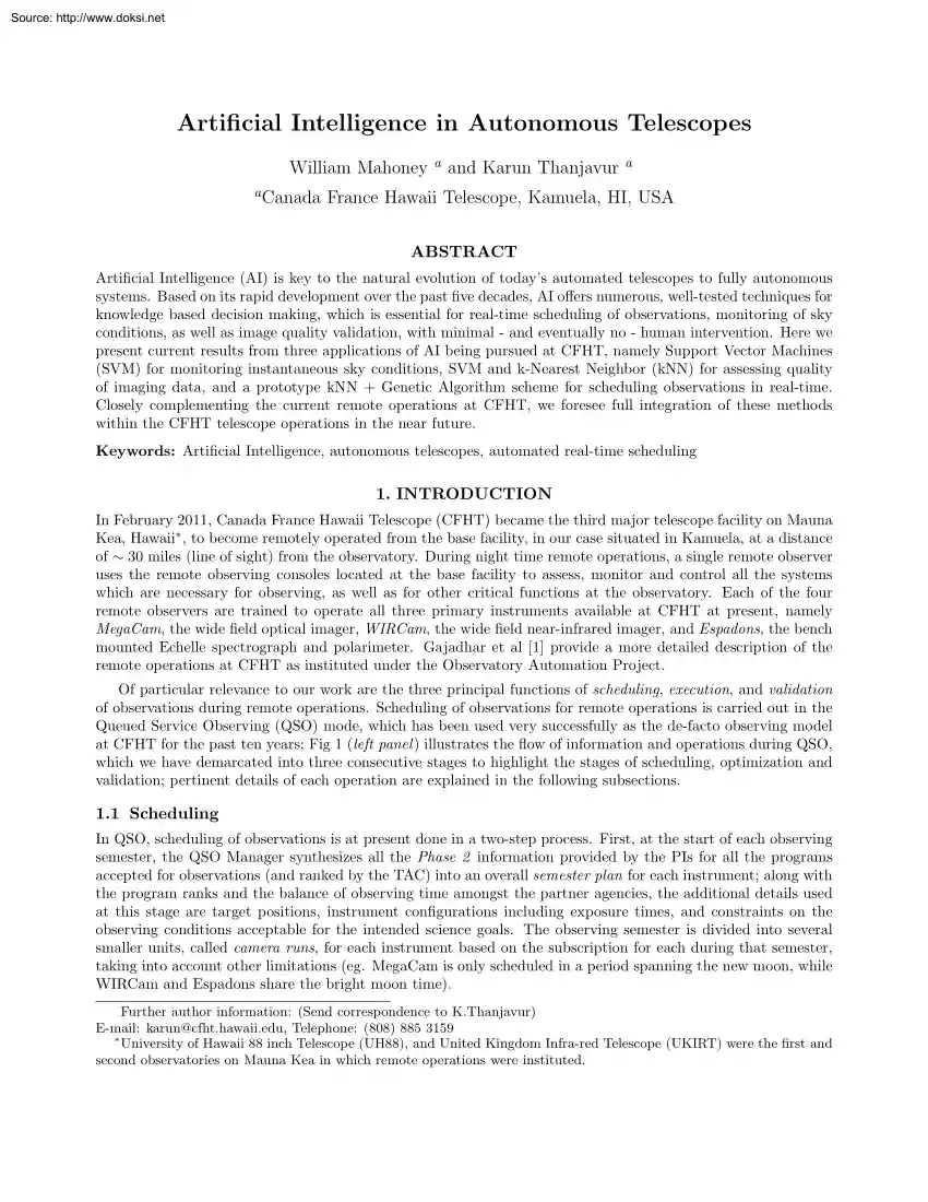
bench mounted Echelle spectrograph and polarimeter. Gajadhar et al [1] provide a more detailed description of the remote operations at CFHT as instituted under the Observatory Automation Project. Of particular relevance to our work are the three principal functions of scheduling, execution, and validation of observations during remote operations. Scheduling of observations for remote operations is carried out in the Queued Service Observing (QSO) mode, which has been used very successfully as the de-facto observing model at CFHT for the past ten years; Fig 1 (left panel ) illustrates the flow of information and operations during QSO, which we have demarcated into three consecutive stages to highlight the stages of scheduling, optimization and validation; pertinent details of each operation are explained in the following subsections. 1.1 Scheduling In QSO, scheduling of observations is at present done in a two-step process. First, at the start of each observing semester, the QSO
Manager synthesizes all the Phase 2 information provided by the PIs for all the programs accepted for observations (and ranked by the TAC) into an overall semester plan for each instrument; along with the program ranks and the balance of observing time amongst the partner agencies, the additional details used at this stage are target positions, instrument configurations including exposure times, and constraints on the observing conditions acceptable for the intended science goals. The observing semester is divided into several smaller units, called camera runs, for each instrument based on the subscription for each during that semester, taking into account other limitations (eg. MegaCam is only scheduled in a period spanning the new moon, while WIRCam and Espadons share the bright moon time). Further author information: (Send correspondence to K.Thanjavur) E-mail: karun@cfht.hawaiiedu, Telephone: (808) 885 3159 ∗ University of Hawaii 88 inch Telescope (UH88), and United Kingdom
Infra-red Telescope (UKIRT) were the first and second observatories on Mauna Kea in which remote operations were instituted. Source: http://www.doksinet Based on this semester plan, each day the Queue Coordinator (QC) on duty prepares several queues for observation during night time operations. Each queue is built of several observational blocks, observing groups (OG) drawn from one or more PI programs. Each queue is designed for different forecast sky conditions during the coming night, measured mainly using the image quality (IQ), sky background, and cloud cover (photometric skies). Naturally, each queue only contains OGs from programs which can accept these sky conditions (as set forth by the PI in Phase 2). 1.2 Optimization At night, the remote observer (RO) chooses the particular queue to observe based on an assessment of the actual sky conditions. In order to provide the information needed for this assessment, the observatory has several weather and sky monitoring systems,
such as MKAM, ASIVA † and SkyCam. As sky and weather conditions change throughout the night, the RO may move freely between queues, constantly optimizing the best OG to observe at any given time commensurate with the prevailing conditions. This optimization is based not only the current observing conditions, but may incorporate other semester specific constraints, such as agency balance. In other words, the RO (usually in consultation with the QC) has the freedom to modify or replace the prepared queues, and pick OGs in real time to maximize the returns from the observations. In ASO, we propose to use a similar approach of real time scheduling, albeit by a suitable AI-based technique; it is important to emphasize that there will be no prepared queues. A Genetic Algorithm optimizes the ’most fit’ OG to be observed from the set selected by a knowledge based system, such as an Artificial Neural Network (ANN). Details of our proposed scheduling model are described in Section 2 1.3
Validation During observations, as soon as each exposure is completed and read out, the observer assesses the data quality using a variety of tools. This involves visual examination on a display tool such as ds9, along with assessment of observing conditions, such as IQ, attenuation and sky background, either measured directly on the image, or obtained directly from analysis processes, such as Realtime. These indicators are compared against the corresponding values specified by the PI in Phase 2. Based on this comparison, the RO assigns a grade to the exposure (ranging from 1 to 5 in order of decreasing quality). Further, based on the grade assigned, the RO validates that exposure. If the exposure is validated, the RO moves to the next observation However, if the exposure is not validated due to poor quality, the RO has to repeat the exposure. Depending on conditions and/or circumstances, the exposure may be repeated either immediately (before the end of the OG), or at some other later
time, either during the current night, or even in succeeding nights when conditions improve. On the following morning, the QC re-examines every exposure for data quality, taking into account the ROs assessment of it during the night. For the majority of the observations, the QC merely accepts the RO’s assessment. However, for observations taken under challenging observing conditions or for reasons based on the semester plan, the QC may revise both the grade and validation status. For example, even in a high ranked program needing pristine seeing, an exposure with IQ grade =3 (normally repeated) may be validated and not repeated perhaps because it is the last day of a camera run and the target is no longer accessible in the next one. The point to be emphasized here is that there is a certain degree of “fuzziness” in both the grading and the validation of exposures. Grading and validating exposures are governed by a set of rules enacted by the QSO Team. Two illustrative examples
are: for IQ, 15% above constraint is normally accepted as Grade=1 and validated, unless the PI has set a hard limit, in which case it is not validated and has to be repeated (for a A ranked program) but may be validated with Grade=2 for a lower ranked program. Similarly, for absorption, all exposures with absorption ¿ 0.12mag are Graded 2 for A-programs and repeated, while they are Graded 1 for other ranks and not repeated (this rule too may be bent depending on circumstances). To summarize, grading and validation are governed by a well designed and comprehensive set of rules, but the QSO Team (RO and QC) may decide to override them under particular circumstances due to extraneous constraints. It is this ‘fuzziness’ in this process that makes it difficult, if not impossible, to implement using standard hard-coded rule structure (using if-then statements, for example), and is suited for knowledge based methods available in AI. † AI based real time assessment of ASIVA images for
photometric sky conditions is described in Section Source: http://www.doksinet Figure 1. (left) The current QSO model showing the flow of information from the PI through the QSO process to the execution of the observations. The three principal stages described in subsections 11 - 13 are shown demarcated for clarity. (right) The current features of our proposed ASO model, which incorporates all three stages of QSO into a single step carried out in realtime. The current prototype includes a kNN selection stage (1), a genetic algorithm for optimization (2), a SVM based tool for validation (3); eventually, each process will have its own self-learning loop (4) to integrate the system’s ‘experience’ into the scheduling process. 1.4 Proposed ASO model In Automated Scheduled Observations (ASO), the observing model we propose is to merge the two-step scheduling process, semester plan + daily queues, described in Sec 1.1, into one step by selecting in realtime the OG to be observed. A
schematic of the proposed ASO model is shown in Fig ?? (right panel ) This machine-based decision will take into consideration not only the instantaneous sky and weather conditions, but also optimize for overall semester plans such as completion rates and agency balances (indicated by the large red rectangle in Fig ?? ). The selection process in the prototype is a kNN classifier, numbered 1 and described in §21 The list of kNN selected OGs is then optimized by a Genetic Algorithm (numbered 2, see §2.2 for details) The optimization process, done in QSO by the RO during observations using the prepared queues, will thus become part of the machine based realtime scheduling in ASO. Finally, the grading and validation (box 3), done in realtime by a heuristic scheme as described in §2.3, will provide the essential feedback loop for the scheduling and optimization; thus, if an observed OG is fully validated, it is removed from the pool of available OGs for the next scheduling step, while if
it is not validated may be treated with higher priority. The kNN selection process, and the Support Vector machine (SVM) used for grading, are both supervised learning schemes, and the ongoing training processes of these are shown schematically by boxes 4; the training is done offline at present, but will be implemented as part of the realtime process in due course. 2. AUTONOMOUS SCHEDULING 2.1 Select the suitable observations with a K-nearest neighborhood algorithm CFHT’s standard Queue Scheduled Observations, QSO, requires creating queues of Observation Groups (OG) binned against potential constraints. Each night a queue will be created which includes OGs requiring photometric conditions, a dark sky background, and excellent seeing conditions (IQ ≤ 05500 ) Additionally, another queue will be populated with OGs with less strict observing constraints – softer seeing, non-photometric skies, bright sky background, etc. Other queues are generated to match all the constraints
between the best and worst possible observing conditions. During the night, the observing staff chooses observations from these queues that best match the conditions the skies are providing. While under manual control, the observer is responsible for matching as closely as possible the sky and atmospheric conditions to the constraints defined for the queued OGs. The observer will know or can determine if it is suitable to observe OGs out of constraint, and by how much they can push these constraints. A computer, using standard top-down deterministic boolean logic, cannot readily make similar decisions. With the performance capabilities of current computing systems, the availability of real-time sky and atmospheric conditions, the Source: http://www.doksinet Figure 2. (left) The observational constraints used as features in the training set for the the KNN fuzzy constraint selection; in this example, the chosen features are airmass, IQ and photometric conditions, as explained in
§2.1 (right) Using integer values, the feature space is mapped into a knowledge map, with each observation represented by a vector of integers (in 3D space in this example), and each vector is associated to a class (observe = Yes or No). In this multi-dimensional space, distances to neighbors may then be measured using a suitable metric, in this example using Euclidean distances. knowledge of historical observations, and the required goals of current and future observing sessions, a computer can be trained to estimate beyond hard-constraint satisfaction – fuzzy selections. The k-Nearest Neighborhood algorithm (KNN) is a computer processing method that can be used for supervised pattern classification, and thus for selection. An n-dimensional training set is mapped to a feature space Subsequent queries of this feature space yield classifications based on distances from the queried feature data and its k nearest neighbors within the knowledge map. The KNN algorithm is used in the
prototype due to ease and rapidness of implementation – it might not be the most suitable AI technique for this application and great care must be used with the training set. A poorly trained KNN is prone to performance issues relating to accuracy and computer response time. Our prototype kNN considers three observing constraints, termed features : airmass, IQ, and photometric conditions. A feature space is generated to map the combinations of these constraints with an expected result This knowledge map represents whether an OG is observable or not, depending on the constraint satisfaction. With this knowledge map, it is possible to map previously unknown, unencountered, or out-of-bounds conditions to a result. Figure 2 (left panel ) depicts a set of observations, their constraint-satisfaction states, and whether or not the observation should be observed with its current state. The prototype loosely attempts to follow guidance from CFHT’s current observing practices. Additionally,
the prototype feature space only considers OGs defined with photometric sky requirements. Ultimately, the feature space and knowledge map will be expanded and made more precise. The feature space must be mapped to a coordinate system of the same dimensionality. In the prototype, three constraints are considered, and are therefore mapped into a three dimensional coordinate system. The mapping process must map the various states of each feature into corresponding numerical values. The values associated to these features must be chosen so that distinction and separation between the classifications is evident. In Figure 2 (right panel ), the feature space has been mapped to integer values, and a particular observation is represented by the vector of those integer values. Each vector is then associated to a class (observe = Yes or No). For the airmass, ‘Conditions Met’ is mapped to 0, ‘Conditions Met up to 15% out of bounds’ has been mapped to 1, and ‘Conditions Not Met’ has
been mapped to 2. The IQ constraint shares a similar mapping The photometric constraint is simply mapped to 0 for photometric and 1 for non-photometric. In the future, it might be possible to map photometric constraints to a sky extinction value. With the feature space mapped to a numerical knowledge map, an OG’s observability based on these three constraints can be estimated using the k-nearest neighborhood algorithm. For example, if an OG was 10% out of Source: http://www.doksinet Figure 3. (left) A sample test case for the kNN classifier showing all the accessible OGs at a particular time plotted on an all-sky image (= 725 images in this example), and color coded by program ranking (A rank = blue; B = red; C and Snapshot = yellow). (right) Using three features, airmass, IQ and photometric conditions, the kNN classifier efficiently selects a subset of 15 OGs, which form the input to the Genetic Algorithm optimization stage to select the ‘most fit’ OG, as described in §2.2
airmass and IQ constraint but under photometric conditions, would it be observable? We map the data such that 10% is 1/3 less than 15%, implying a mapped value of 0.667 (1/3 less than 1, which is representative of 15% out of constraint for Airmass and IQ). Since the assumption is that we are under photometric conditions, we can finish mapping the OG to a point in our knowledge map (0.667, 0667, 00) The prototype KNN implementation now will seek the three nearest neighbors, based on Euclidean distance, in the predefined knowledge map and then compute the resulting class as the maximum of the classes of those three neighbors. In this example, the three closest neighbors to (0.667, 0667, 0) are (0,1,0), (1,0,0), and (1,1,), representing the feature space of Observation 1, Observation 7, and Observation 9. The maximum classification of these three neighbors is Observe=YES Hence, this OG represented in the knowledge map by (0.667, 0667, 00) is suitable for observation Every observing
semester CFHT is provided with thousands of OGs and their associated constraints. For each observing moment throughout the night, any automated system must be able to select the best observation to schedule. This is shown in Fig 22 (left panel ) in which all the accessible OGs are plotted on an all-sky image (from ASIVA, see §2.4), color coded by program ranking ; the clustering of OGs in certain parts of the sky in this example is due only to a high ranked survey-mode program; normally, individual PI programs may be scattered at various sky positions. In this particular example, there are 725 OGs accessible at this time All these accessible OGs are then processed by the kNN classifier, which uses the feature map to classify them as observable or not. The kNN algorithm is designed to efficiently reduce the significant number of suitable observations, nominally several hundreds, to a more manageable set of data, which then forms the input to the optimizer. In this example, the kNN
selected 15 OGs suitable for observation at this time It must be emphasized that in this prototype, only three features have been used whereas in reality the feature space spans seven or more dimensions including important predefined scheduling constraints. 2.2 A Genetic Algorithm optimizer Although the kNN classifier has greatly reduced the large set of OGs to those suitable for this moment (based on current conditions), a real-time scheduler must be able to further optimize this set and select a single best OG (as defined by some metric, which is machine independent and set by the QSO Team). As mentioned in § 1.1, these metrics are based on ‘fuzzy’ rules, which may be overridden or changed at any time Therefore, even though it may be possible to complex program using long chained set of traditional top-down boolean logic rules to accomplish the optimization, the process will lack the flexibility to be reprogrammed in realtime - an essential feature in scheduling. A stochastic
optimization method using a Genetic Algorithm (GA) is eminently suited for this role, and is thus our choice. In our prototype scheduler, the implemented GA scheme is fairly basic – internally labeled as mono-generational and greedy, i.e, it simply selects the best fit, and lacks the evolution through multiple generations which is the Source: http://www.doksinet Figure 4. Scatter plot showing just two of the seven features used for training the SV M light [2] classification scheme for image grading and validation. The data plotted represent WIRCam images drawn from the 2011B semester, with the four panels for each of the four program classes used at CFHT. QC validated images are color coded blue, while red points represent images which were not validated. hallmark of a true GA. In the current GA implementation, a gene is simply an OG The chromosomes that make up the gene are the factors used to calculate the fitness of an OG. The fitness of an OG can be based on an allocated
grade and rank, the target pressure, and various observing statistics such as program completion rates, and agency balances. Only grade,rank, and target pressure were used as chromosomes in our prototype As a mono-generational GA, each OG has its fitness value calculated once, and the best fit is chosen immediately. A production level GA will include crossover and mutation, and also evolve multiple generations with the additional consideration of the OG’s selection impact on its and other OGs’ fitness values. 2.3 SVM for grading and validation Image grading and validation form the essential feedback process which governs the passage of observations through ASO. The steps involved in image assessment by the RO and QC in the QSO model have been described in § 1.3 The rules used for image grading and validation are complex, and are based on multiple constraints simultaneously. As an example, Fig 4 shows a scatter plot of WIRCam exposures drawn from the 2010B semester, classified as
validated or not; the classification is based on seven characteristics, of which only two form the axes, while the four panels represent the program ranks. It is clear that the exposures do not neatly fall into two bins due to the ‘gray’ zones between these constraints and due to exposures being validated even while out of constraint. It must be pointed out that this complexity, especially when they have to be applied to every image in realtime, also leads to human error. For example, WIRCam exposures may be as short as 5s, so the RO has to grade and validate an image in less than 15s (including 10s for readout), and thus assess whether a particular exposure needs to be repeated or not. As in the case of the optimization of OGs for observation, it may be possible to encode all the rules associated with grading and validation in a traditional boolean logic based piece of code. However, as it has been emphasized several times in the preceding sections, these rules are modified or
‘bent depending on other constraints; hence these traditional approaches are cumbersome and usually not practical. A machine based grading scheme must be capable of directly learning from real-life data and experience, akin to the training of a new RO or QC - along with learning the necessary rules, the trainee learns from historical records as well as ‘watches over the shoulder’ of a more experienced QSO team member; subsequently, the trainee’s work is supervised, and corrected if necessary, till a satisfactory level of performance is reached. For machine-based grading and validation, a supervised learning scheme such as a Support Vector Machine (SVM), which is our choice at present, mimics this training process, and is capable of constantly improving it performance using previous experience. The availability of nearly ten years of grading and validation data from QSO operations provides a valuable training set for the SVM. In a process similar to that used by the kNN scheme,
described in § 21, the data quality markers such as IQ and sky background on which the grading rules are based are mapped into a multidimensional feature space. In the training set, the QC assigned grade of each image also forms a feature, while Source: http://www.doksinet whether the images was validated or not forms the output classification. Once the SVM has been thus ‘trained’, it is capable of grading and validating images in realtime. Table 1. Results from a representative training stage of the SV M light classifier used for grading and validating images The training set was ∼17,800 images drawn from the 2011B semester. Both QC as well as SVM assigned grades were used during training, and the corresponding expected precision and associated errors in each case, as explained in § 2.3, are listed here. Training results Precision Error QC Data 95.05% 9.04% MC Data 98.93% 1.12% In the current prototype, we define the SVM feature space using the observing
constraints used in QSO to grade an image (IQ, photometric flag, absorption, sky background, airmass, and sky level) along with the QC assigned grade (= a seven dimensional feature space); based on these features along with the QC assigned validation status for these exposures, the SVM ‘learns’ to classify an exposure as validated or not. We use the publicly available SVM implementation, SV M light‡ [2] as our working model. In a typical trial run, the sky conditions, grades and validation status of all the WIRCam images taken in the first five months of the 2010B observing semester (∼17,800 images) were used as the training set. These images had already been graded and validated by the QSO Team, so the validation status of the images were used in the training. SV M light has an inbuilt feature to test the efficacy of the training process by using a bootstrap technique, in which random trial cases drawn from the training set are reclassified and compared against the input
validation flag.The first line in Table. 1 shows mean precision and error window expected of the trained SVM As an additional step, the training was repeated but with all the exposures in the training set re-graded by applying the QSO grading rules strictly (no ‘fuzziness’ was permitted). The SMV was then retrained on this new training set (same sky conditions + new grades), and second line in Table. 1 shows that the precision “improves” by 3% It should be emphasized that this difference is due not only to inconsistencies in the QC grading but also to the presence of ∼1-2% of cases where the grading rules were ‘bent’. Table 2. SV M light test results using 3160 WIRCam images drawn from the last camera run of the 2010B semester The results represent SVM trained using QC and MC assigned grades and validations (QC/MC model), tested on data with the original QC assigned grades and validations, as well as with MC assigned values (QC/MC data), as described §2.3 Test results
QC data MC data QC model 95.15% 84.76% MC model 96.41% 100% Once trained, the SVM was tested on 3160 WIRCam images taken during the last camera run of the semester. These images had not only the QC assigned grade and validations, but were also re-graded and validated by the machine (similar to what was done to the training set). Four comparative tests were carried out, the results of which are listed in Table. 2 QC model represents a SVM trained using QC assigned grades and validations; MC model uses machine assigned values. QC data represents the test cases with QC assigned grades and validations; similarly the MC data represents the re-graded exposures. The most representative result is the 95% accuracy obtained with the QC-trained QC-tested case, since this incorporates the ‘fuzziness’ used in this process. It is not surprising that the MC-trained MC-tested case returns 100% accuracy, since the grading-validation rules are strictly applied. The worst performance was when
the QC-trained SVM was tested on the strict MC graded test case, since the training included ‘fuzziness’ while the test was strictly enforced. Surprisingly, in the last case of ‡ http://svmlight.joachimsorg/ Source: http://www.doksinet Figure 5. (left) ASIVA difference images showing photometric conditions (top), and non-photometric, cloud cover (bottom); shown alongside each is the distribution of the pixel values in the difference image, and a gaussian fit to it (right) SV M light classification of an ASIVA image following the training process described in §2.4 MC-trained SVM, which did not experience any ‘fuzziness’ during training, is still able to score ∼96% accuracy on test data with out of constraint validations; we are investigating how this surprising performance is achieved. 2.4 SVM for classification of ASIVA images CFHT operates and maintains, ASIVA, an all-sky mid-IR camera atop Mauna Kea. The camera provides zerolight visibility of every cloud
condition, including the very high and cold cirrus As CFHT now operates remotely, real-time data from the device is critical to observers. The device operates during the night, acquiring images in continuous three minute batches. The data we focus on for this exercise is the 10-12µ filter images. Within each three minute batch, eight to ten images of the 10-12µ filter are acquired. A time-based differential image utilizing subtraction of the first from the last image will create a result image that shows any cloud structure, or device noise. In Fig 5, (left panel ), two example difference images are presented. The first image is a photometric sky, the unmasked data is simply the array noise. The second image is obvious non-photometric conditions with significant cloud coverage An observer, using these difference images, can readily identify photometric versus cloudy conditions. Additionally, using the difference image, the observer would be able to identify specific regions in the
sky that are photometric. The point of using AI is to have the machine make this determination So, how can we quantify or formulate this data in a way a machine will understand? Fig 5 also provides how we choose to do this by fitting a Gaussian to the distribution of pixel values of the difference image. The Gaussian fit indicates obvious differences, and now we have a known pattern, which are simply the three coefficients of the Gaussian. Now, we are faced with teaching a computer how to make decisions based on this data. For the CFHT prototype, the Support Vector Machine (SVM) method is employed. A SVM is an artificial intelligence method that utilizes supervised learning for binary pattern classification. The patterns we wish to classify are photometric and not. Using SV M light software§ [2], we trained an SVM with 200 Gaussian coefficients of photometric conditions and 200 Gaussian coefficients of cloudy conditions. An SVM model resulted with a reported 9275% precision. To test
the accuracy of the SVM model, we attempt to classify the original training set of data, and it yielded 97.7% accuracy The model and classification process is now integrated into the real-time processing pipeline of the mid-IR data. And the processing is done so that we can estimate the photometric conditions of smaller than all-sky regions (see right panel, Fig 5). The current processing is able to estimate the photometric conditions of four quadrants of the sky above and below two airmasses. § http://svmlight.joachimsorg/ Source: http://www.doksinet ACKNOWLEDGMENTS We gratefully acknowledge the organizers of the T elescopesf romAf ar conference for having hosted this very relevant gathering and for having provided a platform to share plans and projects in progress along with results from completed work. REFERENCES [1] Gajadhar, S., “Implementation of oap at cfht,” in [These proceedings], SOC, T, ed (2011) [2] Joachims, T., “Making large-scale svm learning practical,” in
[Advances in Kernel Methods - Support Vector Learning], Schölkopf, B., Burges, C, and Smola, A, eds, 53–71, MIT-Press, Dordrecht (1999)
operations at CFHT, we foresee full integration of these methods within the CFHT telescope operations in the near future. Keywords: Artificial Intelligence, autonomous telescopes, automated real-time scheduling 1. INTRODUCTION In February 2011, Canada France Hawaii Telescope (CFHT) became the third major telescope facility on Mauna Kea, Hawaii∗ , to become remotely operated from the base facility, in our case situated in Kamuela, at a distance of ∼ 30 miles (line of sight) from the observatory. During night time remote operations, a single remote observer uses the remote observing consoles located at the base facility to assess, monitor and control all the systems which are necessary for observing, as well as for other critical functions at the observatory. Each of the four remote observers are trained to operate all three primary instruments available at CFHT at present, namely MegaCam, the wide field optical imager, WIRCam, the wide field near-infrared imager, and Espadons, the
bench mounted Echelle spectrograph and polarimeter. Gajadhar et al [1] provide a more detailed description of the remote operations at CFHT as instituted under the Observatory Automation Project. Of particular relevance to our work are the three principal functions of scheduling, execution, and validation of observations during remote operations. Scheduling of observations for remote operations is carried out in the Queued Service Observing (QSO) mode, which has been used very successfully as the de-facto observing model at CFHT for the past ten years; Fig 1 (left panel ) illustrates the flow of information and operations during QSO, which we have demarcated into three consecutive stages to highlight the stages of scheduling, optimization and validation; pertinent details of each operation are explained in the following subsections. 1.1 Scheduling In QSO, scheduling of observations is at present done in a two-step process. First, at the start of each observing semester, the QSO
Manager synthesizes all the Phase 2 information provided by the PIs for all the programs accepted for observations (and ranked by the TAC) into an overall semester plan for each instrument; along with the program ranks and the balance of observing time amongst the partner agencies, the additional details used at this stage are target positions, instrument configurations including exposure times, and constraints on the observing conditions acceptable for the intended science goals. The observing semester is divided into several smaller units, called camera runs, for each instrument based on the subscription for each during that semester, taking into account other limitations (eg. MegaCam is only scheduled in a period spanning the new moon, while WIRCam and Espadons share the bright moon time). Further author information: (Send correspondence to K.Thanjavur) E-mail: karun@cfht.hawaiiedu, Telephone: (808) 885 3159 ∗ University of Hawaii 88 inch Telescope (UH88), and United Kingdom
Infra-red Telescope (UKIRT) were the first and second observatories on Mauna Kea in which remote operations were instituted. Source: http://www.doksinet Based on this semester plan, each day the Queue Coordinator (QC) on duty prepares several queues for observation during night time operations. Each queue is built of several observational blocks, observing groups (OG) drawn from one or more PI programs. Each queue is designed for different forecast sky conditions during the coming night, measured mainly using the image quality (IQ), sky background, and cloud cover (photometric skies). Naturally, each queue only contains OGs from programs which can accept these sky conditions (as set forth by the PI in Phase 2). 1.2 Optimization At night, the remote observer (RO) chooses the particular queue to observe based on an assessment of the actual sky conditions. In order to provide the information needed for this assessment, the observatory has several weather and sky monitoring systems,
such as MKAM, ASIVA † and SkyCam. As sky and weather conditions change throughout the night, the RO may move freely between queues, constantly optimizing the best OG to observe at any given time commensurate with the prevailing conditions. This optimization is based not only the current observing conditions, but may incorporate other semester specific constraints, such as agency balance. In other words, the RO (usually in consultation with the QC) has the freedom to modify or replace the prepared queues, and pick OGs in real time to maximize the returns from the observations. In ASO, we propose to use a similar approach of real time scheduling, albeit by a suitable AI-based technique; it is important to emphasize that there will be no prepared queues. A Genetic Algorithm optimizes the ’most fit’ OG to be observed from the set selected by a knowledge based system, such as an Artificial Neural Network (ANN). Details of our proposed scheduling model are described in Section 2 1.3
Validation During observations, as soon as each exposure is completed and read out, the observer assesses the data quality using a variety of tools. This involves visual examination on a display tool such as ds9, along with assessment of observing conditions, such as IQ, attenuation and sky background, either measured directly on the image, or obtained directly from analysis processes, such as Realtime. These indicators are compared against the corresponding values specified by the PI in Phase 2. Based on this comparison, the RO assigns a grade to the exposure (ranging from 1 to 5 in order of decreasing quality). Further, based on the grade assigned, the RO validates that exposure. If the exposure is validated, the RO moves to the next observation However, if the exposure is not validated due to poor quality, the RO has to repeat the exposure. Depending on conditions and/or circumstances, the exposure may be repeated either immediately (before the end of the OG), or at some other later
time, either during the current night, or even in succeeding nights when conditions improve. On the following morning, the QC re-examines every exposure for data quality, taking into account the ROs assessment of it during the night. For the majority of the observations, the QC merely accepts the RO’s assessment. However, for observations taken under challenging observing conditions or for reasons based on the semester plan, the QC may revise both the grade and validation status. For example, even in a high ranked program needing pristine seeing, an exposure with IQ grade =3 (normally repeated) may be validated and not repeated perhaps because it is the last day of a camera run and the target is no longer accessible in the next one. The point to be emphasized here is that there is a certain degree of “fuzziness” in both the grading and the validation of exposures. Grading and validating exposures are governed by a set of rules enacted by the QSO Team. Two illustrative examples
are: for IQ, 15% above constraint is normally accepted as Grade=1 and validated, unless the PI has set a hard limit, in which case it is not validated and has to be repeated (for a A ranked program) but may be validated with Grade=2 for a lower ranked program. Similarly, for absorption, all exposures with absorption ¿ 0.12mag are Graded 2 for A-programs and repeated, while they are Graded 1 for other ranks and not repeated (this rule too may be bent depending on circumstances). To summarize, grading and validation are governed by a well designed and comprehensive set of rules, but the QSO Team (RO and QC) may decide to override them under particular circumstances due to extraneous constraints. It is this ‘fuzziness’ in this process that makes it difficult, if not impossible, to implement using standard hard-coded rule structure (using if-then statements, for example), and is suited for knowledge based methods available in AI. † AI based real time assessment of ASIVA images for
photometric sky conditions is described in Section Source: http://www.doksinet Figure 1. (left) The current QSO model showing the flow of information from the PI through the QSO process to the execution of the observations. The three principal stages described in subsections 11 - 13 are shown demarcated for clarity. (right) The current features of our proposed ASO model, which incorporates all three stages of QSO into a single step carried out in realtime. The current prototype includes a kNN selection stage (1), a genetic algorithm for optimization (2), a SVM based tool for validation (3); eventually, each process will have its own self-learning loop (4) to integrate the system’s ‘experience’ into the scheduling process. 1.4 Proposed ASO model In Automated Scheduled Observations (ASO), the observing model we propose is to merge the two-step scheduling process, semester plan + daily queues, described in Sec 1.1, into one step by selecting in realtime the OG to be observed. A
schematic of the proposed ASO model is shown in Fig ?? (right panel ) This machine-based decision will take into consideration not only the instantaneous sky and weather conditions, but also optimize for overall semester plans such as completion rates and agency balances (indicated by the large red rectangle in Fig ?? ). The selection process in the prototype is a kNN classifier, numbered 1 and described in §21 The list of kNN selected OGs is then optimized by a Genetic Algorithm (numbered 2, see §2.2 for details) The optimization process, done in QSO by the RO during observations using the prepared queues, will thus become part of the machine based realtime scheduling in ASO. Finally, the grading and validation (box 3), done in realtime by a heuristic scheme as described in §2.3, will provide the essential feedback loop for the scheduling and optimization; thus, if an observed OG is fully validated, it is removed from the pool of available OGs for the next scheduling step, while if
it is not validated may be treated with higher priority. The kNN selection process, and the Support Vector machine (SVM) used for grading, are both supervised learning schemes, and the ongoing training processes of these are shown schematically by boxes 4; the training is done offline at present, but will be implemented as part of the realtime process in due course. 2. AUTONOMOUS SCHEDULING 2.1 Select the suitable observations with a K-nearest neighborhood algorithm CFHT’s standard Queue Scheduled Observations, QSO, requires creating queues of Observation Groups (OG) binned against potential constraints. Each night a queue will be created which includes OGs requiring photometric conditions, a dark sky background, and excellent seeing conditions (IQ ≤ 05500 ) Additionally, another queue will be populated with OGs with less strict observing constraints – softer seeing, non-photometric skies, bright sky background, etc. Other queues are generated to match all the constraints
between the best and worst possible observing conditions. During the night, the observing staff chooses observations from these queues that best match the conditions the skies are providing. While under manual control, the observer is responsible for matching as closely as possible the sky and atmospheric conditions to the constraints defined for the queued OGs. The observer will know or can determine if it is suitable to observe OGs out of constraint, and by how much they can push these constraints. A computer, using standard top-down deterministic boolean logic, cannot readily make similar decisions. With the performance capabilities of current computing systems, the availability of real-time sky and atmospheric conditions, the Source: http://www.doksinet Figure 2. (left) The observational constraints used as features in the training set for the the KNN fuzzy constraint selection; in this example, the chosen features are airmass, IQ and photometric conditions, as explained in
§2.1 (right) Using integer values, the feature space is mapped into a knowledge map, with each observation represented by a vector of integers (in 3D space in this example), and each vector is associated to a class (observe = Yes or No). In this multi-dimensional space, distances to neighbors may then be measured using a suitable metric, in this example using Euclidean distances. knowledge of historical observations, and the required goals of current and future observing sessions, a computer can be trained to estimate beyond hard-constraint satisfaction – fuzzy selections. The k-Nearest Neighborhood algorithm (KNN) is a computer processing method that can be used for supervised pattern classification, and thus for selection. An n-dimensional training set is mapped to a feature space Subsequent queries of this feature space yield classifications based on distances from the queried feature data and its k nearest neighbors within the knowledge map. The KNN algorithm is used in the
prototype due to ease and rapidness of implementation – it might not be the most suitable AI technique for this application and great care must be used with the training set. A poorly trained KNN is prone to performance issues relating to accuracy and computer response time. Our prototype kNN considers three observing constraints, termed features : airmass, IQ, and photometric conditions. A feature space is generated to map the combinations of these constraints with an expected result This knowledge map represents whether an OG is observable or not, depending on the constraint satisfaction. With this knowledge map, it is possible to map previously unknown, unencountered, or out-of-bounds conditions to a result. Figure 2 (left panel ) depicts a set of observations, their constraint-satisfaction states, and whether or not the observation should be observed with its current state. The prototype loosely attempts to follow guidance from CFHT’s current observing practices. Additionally,
the prototype feature space only considers OGs defined with photometric sky requirements. Ultimately, the feature space and knowledge map will be expanded and made more precise. The feature space must be mapped to a coordinate system of the same dimensionality. In the prototype, three constraints are considered, and are therefore mapped into a three dimensional coordinate system. The mapping process must map the various states of each feature into corresponding numerical values. The values associated to these features must be chosen so that distinction and separation between the classifications is evident. In Figure 2 (right panel ), the feature space has been mapped to integer values, and a particular observation is represented by the vector of those integer values. Each vector is then associated to a class (observe = Yes or No). For the airmass, ‘Conditions Met’ is mapped to 0, ‘Conditions Met up to 15% out of bounds’ has been mapped to 1, and ‘Conditions Not Met’ has
been mapped to 2. The IQ constraint shares a similar mapping The photometric constraint is simply mapped to 0 for photometric and 1 for non-photometric. In the future, it might be possible to map photometric constraints to a sky extinction value. With the feature space mapped to a numerical knowledge map, an OG’s observability based on these three constraints can be estimated using the k-nearest neighborhood algorithm. For example, if an OG was 10% out of Source: http://www.doksinet Figure 3. (left) A sample test case for the kNN classifier showing all the accessible OGs at a particular time plotted on an all-sky image (= 725 images in this example), and color coded by program ranking (A rank = blue; B = red; C and Snapshot = yellow). (right) Using three features, airmass, IQ and photometric conditions, the kNN classifier efficiently selects a subset of 15 OGs, which form the input to the Genetic Algorithm optimization stage to select the ‘most fit’ OG, as described in §2.2
airmass and IQ constraint but under photometric conditions, would it be observable? We map the data such that 10% is 1/3 less than 15%, implying a mapped value of 0.667 (1/3 less than 1, which is representative of 15% out of constraint for Airmass and IQ). Since the assumption is that we are under photometric conditions, we can finish mapping the OG to a point in our knowledge map (0.667, 0667, 00) The prototype KNN implementation now will seek the three nearest neighbors, based on Euclidean distance, in the predefined knowledge map and then compute the resulting class as the maximum of the classes of those three neighbors. In this example, the three closest neighbors to (0.667, 0667, 0) are (0,1,0), (1,0,0), and (1,1,), representing the feature space of Observation 1, Observation 7, and Observation 9. The maximum classification of these three neighbors is Observe=YES Hence, this OG represented in the knowledge map by (0.667, 0667, 00) is suitable for observation Every observing
semester CFHT is provided with thousands of OGs and their associated constraints. For each observing moment throughout the night, any automated system must be able to select the best observation to schedule. This is shown in Fig 22 (left panel ) in which all the accessible OGs are plotted on an all-sky image (from ASIVA, see §2.4), color coded by program ranking ; the clustering of OGs in certain parts of the sky in this example is due only to a high ranked survey-mode program; normally, individual PI programs may be scattered at various sky positions. In this particular example, there are 725 OGs accessible at this time All these accessible OGs are then processed by the kNN classifier, which uses the feature map to classify them as observable or not. The kNN algorithm is designed to efficiently reduce the significant number of suitable observations, nominally several hundreds, to a more manageable set of data, which then forms the input to the optimizer. In this example, the kNN
selected 15 OGs suitable for observation at this time It must be emphasized that in this prototype, only three features have been used whereas in reality the feature space spans seven or more dimensions including important predefined scheduling constraints. 2.2 A Genetic Algorithm optimizer Although the kNN classifier has greatly reduced the large set of OGs to those suitable for this moment (based on current conditions), a real-time scheduler must be able to further optimize this set and select a single best OG (as defined by some metric, which is machine independent and set by the QSO Team). As mentioned in § 1.1, these metrics are based on ‘fuzzy’ rules, which may be overridden or changed at any time Therefore, even though it may be possible to complex program using long chained set of traditional top-down boolean logic rules to accomplish the optimization, the process will lack the flexibility to be reprogrammed in realtime - an essential feature in scheduling. A stochastic
optimization method using a Genetic Algorithm (GA) is eminently suited for this role, and is thus our choice. In our prototype scheduler, the implemented GA scheme is fairly basic – internally labeled as mono-generational and greedy, i.e, it simply selects the best fit, and lacks the evolution through multiple generations which is the Source: http://www.doksinet Figure 4. Scatter plot showing just two of the seven features used for training the SV M light [2] classification scheme for image grading and validation. The data plotted represent WIRCam images drawn from the 2011B semester, with the four panels for each of the four program classes used at CFHT. QC validated images are color coded blue, while red points represent images which were not validated. hallmark of a true GA. In the current GA implementation, a gene is simply an OG The chromosomes that make up the gene are the factors used to calculate the fitness of an OG. The fitness of an OG can be based on an allocated
grade and rank, the target pressure, and various observing statistics such as program completion rates, and agency balances. Only grade,rank, and target pressure were used as chromosomes in our prototype As a mono-generational GA, each OG has its fitness value calculated once, and the best fit is chosen immediately. A production level GA will include crossover and mutation, and also evolve multiple generations with the additional consideration of the OG’s selection impact on its and other OGs’ fitness values. 2.3 SVM for grading and validation Image grading and validation form the essential feedback process which governs the passage of observations through ASO. The steps involved in image assessment by the RO and QC in the QSO model have been described in § 1.3 The rules used for image grading and validation are complex, and are based on multiple constraints simultaneously. As an example, Fig 4 shows a scatter plot of WIRCam exposures drawn from the 2010B semester, classified as
validated or not; the classification is based on seven characteristics, of which only two form the axes, while the four panels represent the program ranks. It is clear that the exposures do not neatly fall into two bins due to the ‘gray’ zones between these constraints and due to exposures being validated even while out of constraint. It must be pointed out that this complexity, especially when they have to be applied to every image in realtime, also leads to human error. For example, WIRCam exposures may be as short as 5s, so the RO has to grade and validate an image in less than 15s (including 10s for readout), and thus assess whether a particular exposure needs to be repeated or not. As in the case of the optimization of OGs for observation, it may be possible to encode all the rules associated with grading and validation in a traditional boolean logic based piece of code. However, as it has been emphasized several times in the preceding sections, these rules are modified or
‘bent depending on other constraints; hence these traditional approaches are cumbersome and usually not practical. A machine based grading scheme must be capable of directly learning from real-life data and experience, akin to the training of a new RO or QC - along with learning the necessary rules, the trainee learns from historical records as well as ‘watches over the shoulder’ of a more experienced QSO team member; subsequently, the trainee’s work is supervised, and corrected if necessary, till a satisfactory level of performance is reached. For machine-based grading and validation, a supervised learning scheme such as a Support Vector Machine (SVM), which is our choice at present, mimics this training process, and is capable of constantly improving it performance using previous experience. The availability of nearly ten years of grading and validation data from QSO operations provides a valuable training set for the SVM. In a process similar to that used by the kNN scheme,
described in § 21, the data quality markers such as IQ and sky background on which the grading rules are based are mapped into a multidimensional feature space. In the training set, the QC assigned grade of each image also forms a feature, while Source: http://www.doksinet whether the images was validated or not forms the output classification. Once the SVM has been thus ‘trained’, it is capable of grading and validating images in realtime. Table 1. Results from a representative training stage of the SV M light classifier used for grading and validating images The training set was ∼17,800 images drawn from the 2011B semester. Both QC as well as SVM assigned grades were used during training, and the corresponding expected precision and associated errors in each case, as explained in § 2.3, are listed here. Training results Precision Error QC Data 95.05% 9.04% MC Data 98.93% 1.12% In the current prototype, we define the SVM feature space using the observing
constraints used in QSO to grade an image (IQ, photometric flag, absorption, sky background, airmass, and sky level) along with the QC assigned grade (= a seven dimensional feature space); based on these features along with the QC assigned validation status for these exposures, the SVM ‘learns’ to classify an exposure as validated or not. We use the publicly available SVM implementation, SV M light‡ [2] as our working model. In a typical trial run, the sky conditions, grades and validation status of all the WIRCam images taken in the first five months of the 2010B observing semester (∼17,800 images) were used as the training set. These images had already been graded and validated by the QSO Team, so the validation status of the images were used in the training. SV M light has an inbuilt feature to test the efficacy of the training process by using a bootstrap technique, in which random trial cases drawn from the training set are reclassified and compared against the input
validation flag.The first line in Table. 1 shows mean precision and error window expected of the trained SVM As an additional step, the training was repeated but with all the exposures in the training set re-graded by applying the QSO grading rules strictly (no ‘fuzziness’ was permitted). The SMV was then retrained on this new training set (same sky conditions + new grades), and second line in Table. 1 shows that the precision “improves” by 3% It should be emphasized that this difference is due not only to inconsistencies in the QC grading but also to the presence of ∼1-2% of cases where the grading rules were ‘bent’. Table 2. SV M light test results using 3160 WIRCam images drawn from the last camera run of the 2010B semester The results represent SVM trained using QC and MC assigned grades and validations (QC/MC model), tested on data with the original QC assigned grades and validations, as well as with MC assigned values (QC/MC data), as described §2.3 Test results
QC data MC data QC model 95.15% 84.76% MC model 96.41% 100% Once trained, the SVM was tested on 3160 WIRCam images taken during the last camera run of the semester. These images had not only the QC assigned grade and validations, but were also re-graded and validated by the machine (similar to what was done to the training set). Four comparative tests were carried out, the results of which are listed in Table. 2 QC model represents a SVM trained using QC assigned grades and validations; MC model uses machine assigned values. QC data represents the test cases with QC assigned grades and validations; similarly the MC data represents the re-graded exposures. The most representative result is the 95% accuracy obtained with the QC-trained QC-tested case, since this incorporates the ‘fuzziness’ used in this process. It is not surprising that the MC-trained MC-tested case returns 100% accuracy, since the grading-validation rules are strictly applied. The worst performance was when
the QC-trained SVM was tested on the strict MC graded test case, since the training included ‘fuzziness’ while the test was strictly enforced. Surprisingly, in the last case of ‡ http://svmlight.joachimsorg/ Source: http://www.doksinet Figure 5. (left) ASIVA difference images showing photometric conditions (top), and non-photometric, cloud cover (bottom); shown alongside each is the distribution of the pixel values in the difference image, and a gaussian fit to it (right) SV M light classification of an ASIVA image following the training process described in §2.4 MC-trained SVM, which did not experience any ‘fuzziness’ during training, is still able to score ∼96% accuracy on test data with out of constraint validations; we are investigating how this surprising performance is achieved. 2.4 SVM for classification of ASIVA images CFHT operates and maintains, ASIVA, an all-sky mid-IR camera atop Mauna Kea. The camera provides zerolight visibility of every cloud
condition, including the very high and cold cirrus As CFHT now operates remotely, real-time data from the device is critical to observers. The device operates during the night, acquiring images in continuous three minute batches. The data we focus on for this exercise is the 10-12µ filter images. Within each three minute batch, eight to ten images of the 10-12µ filter are acquired. A time-based differential image utilizing subtraction of the first from the last image will create a result image that shows any cloud structure, or device noise. In Fig 5, (left panel ), two example difference images are presented. The first image is a photometric sky, the unmasked data is simply the array noise. The second image is obvious non-photometric conditions with significant cloud coverage An observer, using these difference images, can readily identify photometric versus cloudy conditions. Additionally, using the difference image, the observer would be able to identify specific regions in the
sky that are photometric. The point of using AI is to have the machine make this determination So, how can we quantify or formulate this data in a way a machine will understand? Fig 5 also provides how we choose to do this by fitting a Gaussian to the distribution of pixel values of the difference image. The Gaussian fit indicates obvious differences, and now we have a known pattern, which are simply the three coefficients of the Gaussian. Now, we are faced with teaching a computer how to make decisions based on this data. For the CFHT prototype, the Support Vector Machine (SVM) method is employed. A SVM is an artificial intelligence method that utilizes supervised learning for binary pattern classification. The patterns we wish to classify are photometric and not. Using SV M light software§ [2], we trained an SVM with 200 Gaussian coefficients of photometric conditions and 200 Gaussian coefficients of cloudy conditions. An SVM model resulted with a reported 9275% precision. To test
the accuracy of the SVM model, we attempt to classify the original training set of data, and it yielded 97.7% accuracy The model and classification process is now integrated into the real-time processing pipeline of the mid-IR data. And the processing is done so that we can estimate the photometric conditions of smaller than all-sky regions (see right panel, Fig 5). The current processing is able to estimate the photometric conditions of four quadrants of the sky above and below two airmasses. § http://svmlight.joachimsorg/ Source: http://www.doksinet ACKNOWLEDGMENTS We gratefully acknowledge the organizers of the T elescopesf romAf ar conference for having hosted this very relevant gathering and for having provided a platform to share plans and projects in progress along with results from completed work. REFERENCES [1] Gajadhar, S., “Implementation of oap at cfht,” in [These proceedings], SOC, T, ed (2011) [2] Joachims, T., “Making large-scale svm learning practical,” in
[Advances in Kernel Methods - Support Vector Learning], Schölkopf, B., Burges, C, and Smola, A, eds, 53–71, MIT-Press, Dordrecht (1999)