Traffic school | Higher education » Avissar-Holder-Abehserra - The Duke University Helicopter Observation Platform

THE DUKE UNIVERSITY HELICOPTER OBSERVATION PLATFORM BY RONI AVISSAR, HEIDI E. HOLDER, N A T H A N ABEHSERRA, M A D A M BOLCH, K . N O V I C K , PATRICK C A N N I N G , KATYA PRINCE, JOSE MAGALHAES, N A O K I MATAYOSHI, G . KATUL, ROBERT L W A L K O , A N D KRISTINA M JOHNSON ^ Duke Universitys modified Jet Ranger helicopter takes advantage of its ability to fly slowly with sensor payloads to make valuable atmospheric measurementsincluding at extremely low altitudes. A s pointed out in many publications (e.g, Avissar and Pielke 1989; Avissar and Schmidt 1998T Schmid 2002; Avissar and Werth 2005; Kim et al. 2006), and also emphasized in a recent report of the National Research Council on integrating multiscale observations of U.S waters (National Research Council 2008), spatial variability of the Earths surface has a considerable impact on the at mo sphere at all scales. Understanding the mecha nisms involved in l a n d - a t m o s p h e r e interactions in this highly

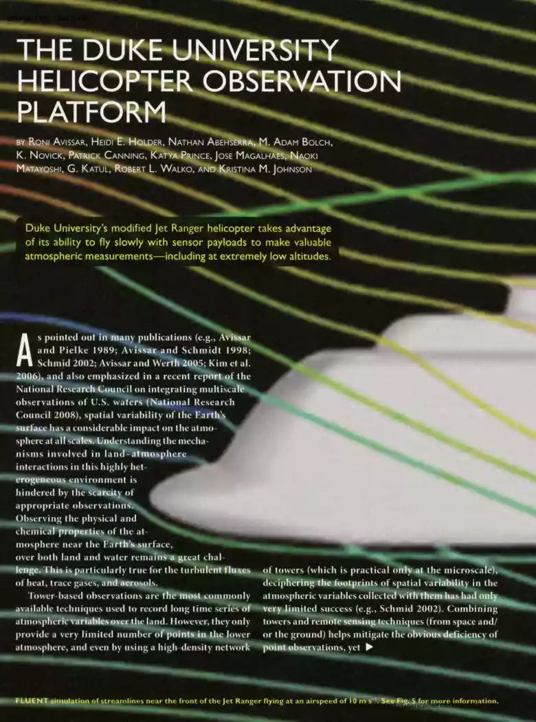
heterogeneous environment is hindered by the scarcity of A app rop r i at e obse r vat ion S. Observing the physical and chemical properties of the atmosphere near the Earths surface, over both land and water remains a great challenge. This is particularly true for the turbulent fluxes of towers (which is practical only at the microscale), of heat, trace gases, and aerosols. deciphering the footprints of spatial variability in the lower-based observations are the most commonly atmospheric variables collected with them has had only available techniques used to record long time series of very limited success (e.g, Schmid 2002) Combining atmospheric variables over the land. However, they only towers and remote sensing techniques (from space and/ provide a very limited number of points in the lower or the ground) helps mitigate the obvious deficiency of atmosphere, and even by using a high-density network point observations, yet • FLUENT simulation of streamlines near the front of the

Jet Ranger flying at an airspeed of 10 m s". See Fig 5 for more information Unauthenticated | Downloaded 05/08/21 12:27 PM UTC many of the processes linking the two methods are empirical in nature, and the fundamental mechanisms needed to use such an approach more efficiently and more accurately remain to be elucidated (Kim et al. 2006) Many different types and sizes of aircraft have been used to make spatiotemporal observations of the atmosphere. Because aircraft have a limited flight-time capability and are expensive to operate, they are used only in relatively short missions, typically as part of dedicated intensive field campaigns. Yet, in spite of these obvious limitations, they fulfill a key role in our observation strategy. An overview of fixed-point versus airborne observations is provided in Muschinski et al. (2001) To fill a gap in our aircraft observation capability, we developed a helicopter observation platform (HOP), based on a Bell 206B3 "Jet Ranger"

(hereafter referred to as the "Duke HOP"). The purpose of this paper is to introduce this platform to the broadly defined atmospheric and oceanic science communities. First, the value of a helicopter platform is discussed. Then, a description of the relevant characteristics of the Jet Ranger for its use as the Duke HOP and of the research sensors mounted permanently on it is provided. Third, analytical and numerical studies, as well as onboard and ground observations, are used to describe its aerodynamic envelope and highlight its AFFILIATIONS: AviSSAR ,* HOLDER, ABEHSERRA, BOLCH, CANNING, MAGALHAES, AND WALKODepartment of Civil and Environmental Engineering, Edmund T. Pratt School of Engineering, Duke University, Durham, N o r t h Carolina; NOVICK AND KATULNicholas School of the Environment, Duke University, Durham, N o r t h Carolina; PRINCEPrince Consulting, LLC, Durham, N o r t h Carolina; MATAYOSHI Japan Aerospace Exploration Agency (JAXA), Tokyo, Japan; JOHNSON +

Department of Electrical and Computer Engineering, Edmund T. Pratt School of Engineering, Duke University, Durham, N o r t h Carolina • C U R R E N T AFFILIATION: Rosenstiel School of Marine and Atmospheric Science (RSMAS), University of Miami, Miami, Florida +CURRENT AFFILIATION: Johns Hopkins University, Baltimore, Maryland CORRESPONDING A U T H O R : Dr. Roni Avissar, Rosenstiel School of Marine and Atmospheric Science (RSMAS), University of Miami, 4600 Rickenbacker Causeway, Miami, FL 33149-1031 E-mail: ravissar@rsmas.miamiedu The abstract table of for this article can be found in this issue, following contents. DOhlO.I I75/2008BAMS2628I In final form 19 November 2008 2009 American Meteorological Society 940 I BAflS- the operational range for research missions. Finally, we briefly describe the recent research missions in which it was involved as a demonstration of its potential use, and the current improvements being made to it for upcoming research missions. FILLING A

GAP IN AIRCRAFT PLATFORMS. In general, large airplanes have expensive costs for fuel, maintenance, and personnel, but they house a full complement of scientific investigators. They have long flight durations, large payloads, and fast transit speeds. However, at the airspeeds needed for large airplanes to maintain lift (at least 60-70 m s 1), "supermicron" particles are sampled very inefficiently due to inlet losses and, as explained in detail below, turbulent fluxes are measured less accurately. While they can fly low (as they do, obviously, on landing and takeoff), it is not practical and is, in fact, a quite risky maneuver outside of an airport environment. Furthermore, as explained in sidebar 1, the U.S Federal Aviation Regulation (FAR; section 91.119) practically prohibits low-level flights (i.e, less than 500 ft AGL) with airplanes over much of the continental United States because it is difficult to find a long enough leg without operating ". closer than 500feet to

any person, vessel, vehicle, or structure." Small airplanes have lower costs, but they also have limitations on duration, speed, and maximum payload. The slower speed (as compared to large airplanes) is an advantage for aerosol sampling and for measuring turbulent fluxes, but it prohibits the use of small airplanes in areas more than -100 km from an airport because the transit time will often require 50% or more of the allowable flight duration. This limitation is particularly relevant for offshore research missions. To alleviate the payload limit, the Network of Airborne Environmental Research Scientists (information available online at www.naersorg) suggests simultaneously using well-coordinated aircraft, each one dedicated to a particular instrument. An important point to note is that there is no distinction in FAR section 91.119 between types of airplanes, and they are all subject to the same altitude restrictions, no matter how small they are. The main advantage of the

helicopter is that is combines slow airspeed and near-surface flight capability (Muschinski et al. 2001; Siebert et al 2006) The importance of slow airspeed measurements, which has been discussed in detail by Siebert et al. (2006), is maybe best illustrated with a realistic example. Assuming that a helicopter flies at an airspeed that is 1/3 that of an airplane (say, 25 versus 75 m s I); it measures atmospheric variables at a spatial resolution JULY 2009 Unauthenticated | Downloaded 05/08/21 12:27 PM UTC FEDERAL AVIATION REGULATION § 91.119 CONCERNING LOW-ALTITUDE FLIGHTS § 91.119 Minimum safe altitudes: General Except w h e n necessary f o r takeoff o r landing, no person may operate an aircraft below the following altitudes: (a) A n y w h e r e . A n altitude allowing, if a p o w e r unit fails, an emergency landing w i t h o u t undue hazard t o persons o r p r o p e r t y on the surface (b) O v e r congested areas. O v e r any congested area of a city, t o w n , o r

settlement, o r over any open air assembly of persons, an altitude of 1,000 feet above the highest obstacle w i t h i n a horizontal radius of 2,000 feet of the aircraft. (c) O v e r o t h e r than congested areas. A n altitude of 500 feet above the surface, except over open w a t e r o r sparsely populated areas. In those cases, the aircraft may not be operated closer than 500 feet t o any person, vessel, vehicle, o r structure. (d) Helicopters. Helicopters may be operated at less than the minimums prescribed in paragraph (b) o r (c) of this section if the operation is conducted w i t h o u t hazard t o persons o r p r o p e r t y on the surface . 3 times higher than that obtained by the airplane if both use the exact same sensors. This is important for measuring the high-frequency turbulent perturbations, which can be an important component of the turbulent fluxes in the atmospheric boundary layer (ABL). The importance of low-altitude flight capability is illustrated in Fig 1,

which shows a characteristic vertical profile of sensible heat flux in the convective boundary layer (CBL). Understandably, an airplane not allowed to fly below the altitude illustrated with the gray line would be limited to sampling the CBL at heights where the absolute value of the flux is near zero. Exacerbated by the loss of accuracy and precision associated with the loss of high-frequency turbulent motions resulting from high airspeed (Siebert et al. 2006), this could result in measurements that generate an error in the flux calculation that is at least of the same magnitude as the flux itself. Given that the sensible heat flux decreases linearly with height in the mixed layer, the entire profile could be assessed from two altitudes, yet minor absolute errors at two altitudes near the CBL top could result in large errors in derived surface fluxes. On the other hand, a sampling just above the atmospheric surface layer and near the top of the CBL results in a much more reliable flux

profile. It is worth noting that during the Cloud and Land Surface Interaction Campaign (CLASIC) in June 2007, surface sensible heat fluxes of less than 30 W m 2 and ABL heights of 200-300 m were frequently observed. Thus, airplane measurements of that variable would not have been very useful given the precision and sampling frequenAMERICAN METEOROLOGICAL SOCIETY FIG. I Schematic profile of turbucy of even the lent sensible heat flux in a typical most sophistiCBL (z. indicates its top) The solid cated, state-ofgrey line illustrates an example of the-art sensors minimum allowed flight altitude currently availfor airplanes. able. A similar case could be made for any turbulent flux that varies with height in the ABL. This is even more crucial when the surface flux is dependent on the land cover type (as is the case for heat, momentum, moisture, C0 2 , and many trace gases and aerosols), in which case it is unrealistic to expect reasonable estimates of turbulent fluxes from airplane

observations. The importance of low-level flights is also very important for the stable boundary layer, which is typically much shallower than the CBL and is often dominated by waves and instabilities, and by small-scale turbulence that is neither homogeneous nor stationary. Lenschow et al. (1994) investigated the errors obtained in flight legs They found that the maximum systematic and random errors could be estimated by 2.2z(z/z)°- 5 /L and 175(z/z)°-25(zJL)° respectively, where z. is the height of the convective boundary layer, z is the flight altitude, and L is the length of the flight leg. Accordingly, they estimated that flying a 4,000-m leg at an altitude of 100 m AGL in a 1,000-m-deep boundary layer resulted in a maximum systematic error of 17% and a maximum random error of 49%. Flying a 10-km leg at a height of 3 m AGL, as we did with the Duke HOP during CLASIC, reduces these theoretical errors (which cannot be reached in real flight conditions) to about 1% and 7%,

respectively. JULY 2009 BAF15- | 9 4 1 Unauthenticated | Downloaded 05/08/21 12:27 PM UTC The helicopter p l a t f o r m can also enjoy an effectively longer duration at the designated sampling area, because it can land and refuel at locations inaccessible to fixed-wing aircraft, removing the waste of fuel and time that occurs in transit. Indeed, it is logistically possible to bring a fuel truck to a landing site at or near the sampling area where the helicopter could stop regularly for refueling. Perhaps the biggest advantage of all, which has been demonstrated with the "Helipod" (a gliding pod towed by a helicopter) described by Muschinski and Wode (1998), is the opportunity to perform marine observations far from shore using a helipad aboard a ship. Such a helipad is available, for instance, on the National Oceanic and Atmospheric Administration (NOAA) David Starr Jordan and could be adapted to fit other research vessels to make remote marine locations requiring a U.S

Class I research ship accessible, with effectively all of the flight hours available on station for the observations. Modern commercial cruisers are also typically equipped with helipads, and cooperation with the scientific community, as is maybe best demonstrated with the past research missions conducted on the Explorer of the Seas (online at www.royalcaribbeancom), is feasible It is therefore conceivable to deploy a properly equipped HOP for marine operation in collaboration with passenger and/or cargo ships. Unlike even large aircraft that can remain on station for a few hours before heading back to shore, a helicopter on a ship could stay at sea for extensive periods, thus providing the opportunity for long marine atmospheric campaigns. The magnitude of turbulent fluxes, aerosols, and atmospheric chemistry above the oceans remain uncertain, and HOP has the potential to revolutionize the quality and quantity of scientific information that could be gathered there. Despite these

advantages, helicopters have been used mostly for remote sensing applications (e.g, Babin 1996), and only sporadically for in situ atmospheric sampling. Maybe this can be attributed to the popular belief in our scientific community that atmospheric sampling on a helicopter is not feasible because of the main rotor "downwash." However, as illustrated in Leishman (2006, e.g, Fig 117, p 661, among many other examples therein) and discussed by Siebert et al. (2006), and below in this article, even at low airspeed the wake created by the main rotor is skewed backward and has practically no impact on the air in front of the helicopter nose. This is why the pitot tube of many helicopters is installed at that location (including on the Jet Ranger) so that even at airspeeds as low at 6-7 m s 1, the rotor wake has 942 no significant impact on the helicopter instrument readings. Obviously, accurate flight instrument readings are essential for flight safety and measuring the rotor wake

instead of the undisturbed atmosphere would be unacceptable. A few observational studies performed on board helicopters are, however, quite noteworthy. Among them, a series of air-sampling campaigns was carried out by the Tennessee Valley Authority (TVA) with a Bell 205 specifically equipped to observe various atmospheric oxidants (e.g, Imhoff et al 1995; Valente et al. 1998; Luria et al 1999, among many others). Air quality monitoring was also conducted by Roeckens et al. (1992), De Saeger et al (1993), and Desmet et al. (1995) Helipod (Muschinski and Wode 1998; Roth et al. 1999; Muschinski et al 2001; and van den Kroonenberg and Bange 2007, among others) and the Airborne Cloud Turbulence Observation System (ACTOS) described by Siebert et al. (2006) are gliding pods towed by helicopters, which are used to sample various atmospheric properties. While these gliding pods benefit from many of the advantages of a helicopter platform (e.g, time on station, operation from ships at sea, low

speed), they restrict some of the maneuverability of the towing helicopter (e.g, flight very near the Earth surface, quick turns). Also, to reduce erratic movements resulting from turbulence, they typically fly into the wind, thus reducing the versatility of experiments that can be conducted with helicopters. For that reason, Helipod is flown at 40 m s 1 (Muschinski et al. 2001) Siebert et al (2006) indicate that ACTOS flies at very low speed (15 m s-1), yet we presume that this is mostly feasible when crosswind turbulence is quite weak. Indeed, it is challenging to maintain a small helicopter straight and level in turbulent air at low airspeeds, let alone with a pod towed under such a helicopter. Motivated by the need for very near-surface observations and the increased accuracy of measurements obtained at low speed, and inspired by the achievements of the above-mentioned research missions performed with helicopters, we developed the Duke HOP. P L A T F O R M D E S C R I P T I O N .

The Jet Ranger adopted for the Duke HOP is a light, single-engine (turbine) helicopter that was originally designed as a light observation helicopter for the U.S Army Its first commercial version was certified in 1966, and while many of its components have been improved over the past 40+ yr, its conceptual design dates back to the early 1960s. It is simple, robust, and nimble, I BAflS- JULY 2009 Unauthenticated | Downloaded 05/08/21 12:27 PM UTC and based on the U.S National Transportation Safety Board (NTSB) statistics, it is the safest, single-engine aircraft (including airplanes!) flying today It has been used extensively by the military and police, for news gathering, and for many other applications all over the world. As a result, it benefits from a very broad international network of technical support. A full description of the Jet Ranger characteristics and performance is available on the manufacturers Web site (www.bellhelicopterscom), and only the most relevant

characteristics for its use as the Duke HOP are summarized in Table 1. While its available payload capability (APC) for scientific instrumentation is limited, when compared to its hourly fuel consumption, it is one of the most efficient turbine helicopters. Thus, it is comparatively cheap to operate, which was another reason (in addition to its safety record and technical support) to adopt it as the Duke HOP. Seats, all unnecessary plastic covers, and soundproofing material were removed f r o m the 40-ft 3 aft cabin to reduce its weight and to make room for instrument and computer racks. This resulted in an increase of the APC by nearly 120 lbs. The copilot/passenger seat in the forward cabin was also eliminated to make room (-18 ft 3 ) for an atmospheric chemistry package (ACP) with inlets going straight through the helicopter nose. 1 There is also a 16-ft 3 baggage compartment located behind the aft cabin that can be exploited for additional instruments and computers, if needed. The

Jet Ranger DC generator provides 105 A (28 V) on a continuous basis (200 A for 5 s and 170 A for 2 min). In its configuration as the Duke HOP with its navigation and communication systems, it uses - 4 2 A in cruise flight, thus leaving up to - 6 3 A for the continuous operation of the research equipment, which consists of a data acquisition system (DAS), instruments, and sensors. Two independent power inverters (from 28 V DC to 110 V AC) provide - 4 KW for the research equipment. The DAS and all instruments and sensors are controlled by switches located in the cockpit and operated by the pilot. 2 Figure 2 shows p i c t u r e s of the H O P as it is currently equipped with its permanent scientific instrumentation, that is, the sensors that are expected to be used for any scientific mission. This set of sensors consists of an Aventech Research, Inc (www aventech.com), Advanced Airborne Measurement 1 Main characteristics and performance of the Duke HOP. The BOW is the weight of the HOP,

including its permanent scientific equipment, fully fueled, and with a 170-lb pilot. The APC (= MGW - BOW) is the maximum weight of the additional scientific equipment that could be loaded on the helicopter, assuming standard meteorological conditions. The Jet Ranger is certificated to a maximum altitude of 20,000 ft. However, for its application as a HOP, it is not practical to fly above 12,000 ft except in special cases. The maximum endurance provided here is based on flights conducted near the ground surface at an airspeed of 30 m s"1 during a hot summer day in Oklahoma. It does not include the 20-min fuel reserve mandated by federal aviation regulations. TABLE 1. Characteristics Duke HOP Maximum gross weight ( M G W ) 3350 lbs Base operating weight ( B O W ) 2900 lbs Additional payload capability (APC) 450 lbs A f t cabin and baggage cargo volume 56 ft 3 Maximum altitude f o r research mission Maximum endurance f o r research mission 12,000 f t 3.67 h Solutions-20

(AIMMS-20) that measures the three components of the wind, temperature, and relative humidity, a Licor (www.licorcom) LI-7500 that measures water vapor and C 0 2 concentrations, and an ultrasonic velocimeter (USV) prototype developed by the Kaijo Sonic Corporation in collaboration with Japan Aerospace Exploration Agency (JAXA; Matayashi et al. 2005) This USV also measures the three components of the wind and the virtual temperature. Because this information is crucial for the calculation of all turbulent fluxes, it is beneficial to have this duplication, especially because the two sensors are based on different technologies. Both the AIMMS-20 and USV have a data output rate of 40 Hz and the Licor has an output rate of 160 Hz, which is reduced to 40 Hz for consistency with the other sensors when calculating fluxes. The AIMMS-20 consists of the following four modules: 1) an air-data probe (located on the nose of the HOP) that senses temperature, humidity, barometric pressure, the

three-dimensional aircraftrelative airflow vector, and the three-axis acceleration and magnetic field measurement; 2) an inertial measurement unit that provides three-axis acceleration T h e ACP, which includes a Proton Transfer Reaction Mass Spectrometer (PTR-MS), is in development stage and is not yet available for research mission. It is expected to become available in s u m m e r 2009 2 T h e first author is the H O P lead investigator and its pilot. AMERICAN METEOROLOGICAL SOCIETY JULY 2009 BAF15- | 9 4 3 Unauthenticated | Downloaded 05/08/21 12:27 PM UTC FIG. 2 (left) Permanent sensors mounted on the Duke HOP, (top right) pilot cockpit, and (bottom right) aft cabin seen from the right and three-axis angular rates; 3) a dual-processor global positioning system that includes dual-antenna inputs for differential carrier-phase measurement (one antenna is located on the nose and the other one is on the tail of the HOP); and 4) a central processing module that, among other

functions, converts the inertial and GPS phase/position/velocity data into precise attitude data (roll, pitch, true heading). This processed information is shared with all other sensors and, therefore, the AIMMS-20 is operated during all research missions. It is also used to coordinate the clock between the different sensors and to trigger data storage (see below). The LI-7500 open path C 0 2 / H 2 0 gas analyzer consists of the following two components: 1) the analyzer sensor head that is mounted on the nose of the HOP, and 2) the control box, which houses the electronics and is located in the aft cabin (Fig. 2) The sensor head has a 12.5-cm open path, with single-pass optics and a large 1-cm-diameter optical beam. Reference filters centered at 3.95 and 240 ^m provide for attenuation corrections at nonabsorbing wavelengths. Absorption at wavelengths centered at 4.26 and 259 ^m provide for measurement of C 0 2 and water vapor, respectively. These features minimize sensitivity to drift

and dust, which can accumulate^during normal operation. The USV is based on a conventional ultrasonic anemometer that consists of two main components: 1) a probe (also located on the nose of the HOP), which senses the three-dimensional aircraft-relative airflow 944 I BAflS- vector and ambient temperature by measuring ultrasonic pulse transit time between three mounts (Fig. 2); and 2) a control box and a junction box (located in the aft cabin), which control ultrasonic pulse emissions and output the measured data via RS-232C. The main advantage of the USV as compared to a pitot-static system is that it can provide accurate measurements at low speeds and in crosswinds. This is obviously important for helicopters Unlike conventional ultrasonic anemometers, the USV uses high-frequency (200 kHz) ultrasonic pulses to reduce acoustic noise, and its probe shape minimizes airflow disturbance at high airspeeds. These modifications allow a broad range of airflow measurements, from 0 to 70 m s

1 which covers the entire flight envelope of the HOR On ACTOS, Siebert et al. (2006) use a state-of-the-art ultrasonic anemometer whose technical characteristics appear to be superior to those of our USV. This anemometer is thoroughly described in Siebert and Muschinski (2001). They also use an ultrafast thermometer (UFT) with a 500-Hz resolution, which is considerably more precise than our temperature sensors. While we are eager to mount the best-available technology on the Duke HOP so that it remains consistently at the cutting edge of measurement performance, we chose our sensors not only for their reasonably good performance but also for their robustness. Our approach is to upgrade the platform with better sensors when they become available and their superior capability can be demonstrated in the harsh environment of low-level flights, where dust, moisture, and especially insects can be a serious problem for fragile sensors. The computer is used to run a National Instruments

LabVIEW (www.nicom/labview) program that reads the data input from each instrument, parses and displays data, and controls the logging of the data to files. The AIMMS-20 and USV communicate via individual RS232 serial lines to the PC. The Licor outputs two 0-10-V analog signals (proportional to water vapor and C0 2 ) that are connected to the PC through a National Instruments USB-6008 data acquisition (DAQ) card. An independent pressure sensor (with its own static port located under the HOP) that is used to calculate potential temperature in real time provides a 0-10-V analog signal that is JULY 2009 Unauthenticated | Downloaded 05/08/21 12:27 PM UTC also wired to the DAQ card. Finally, a 0-5-V signal is fed through a switch in the cockpit and back to the DAQ card so that the pilot can easily mark the beginning and the end of a measurement flight leg by creating a signal in the log file. This is a useful marker when processing the data after the flight. The real-time visualization

that is displayed on the monitor located in the cockpit includes the potential temperature profile, which is calculated from the temperature measured with the USV and the pressure sensor. This real-time profiling capability is useful for the assessment of the height of the various atmospheric layers and, accordingly, for the selection (in real time) of relevant flight altitudes. It also displays the DAS information in graphic form and a series of green/red virtual buttons, indicating the functioning status of the various sensors and instruments. H. E Holder et al (2009a, unpublished manuscript) describe the principles upon which these sensors are based and how their outputs are treated to extract high-frequency atmospheric turbulence variables in more detail. Thus, for brevity, this material is not duplicated here and interested readers are referred to that other publication. It is also important to note that the Duke HOP has a modular design and, therefore, sensors and instruments can

be mounted on it for specific experiments and disconnected afterward. It also has an attachment device under its belly, which includes power and data connectors. Thus, instruments can be mounted inside pods that can be rapidly attached to that universal device and that can communicate with the onboard data acquisition system, if desired. For instance, an aerosol lidar has been constructed in such a pod. It is shown in Fig. 3 and discussed in Eichinger et al (2008). This lidar can be attached to the HOP in a few minutes, and dismounting it is even faster. Finally, it should be mentioned that the Duke HOP is equipped with the Chelton Flight Systems (www. cheltonflightsystems.com), which is a state-of-the-art navigation system that provides three-dimensional synthetic vision of the terrain with all its obstructions (including antennas, buildings, etc.), a complete flight/navigation instrumentation system, and the "Highway-in-the-Sky" ("HITS"), which depicts the

programmable flight track in a perspective-like tunnel. This system helps perform very precise flights according to preset altitudes and coordinates of the path to be flown. It also includes traffic awareness and real-time satellite weather for enhanced safety. It is backed up by a battery-operated portable GPS Garmin 496 (www.garmincom) in case of electrical power loss. AMERICAN METEOROLOGICAL SOCIETY A E R O D Y N A M I C ENVELOPE A N D AIRSPEED O P E R A T I O N . There is abundant professional literature that describes the theory, experiments, and physical and numerical models that have been developed and applied to explain the wake generated by the main rotor and its interactions with the helicopter frame while hovering and in forward flight (e.g, Leishman 2006) However, partly to dispel the above-mentioned "downwash" misconception, and mostly to identify the range of airspeeds that can provide the best results for measuring fluxes and aerosols (which is essential for

research mission planning), we used an analytical model, numerical simulations, and observations collected on board the HOP. These studies are summarized below A N A L Y T I C A L STUDY. Rotor performance in flight was first derived and explained by Glauert (1935) based on the analysis of marine propellers proposed by Rankine (1865) that was further developed by Froude (1878) and Froude (1889). It is often referred to as the "Rankine-Froude momentum theory." It is thoroughly described in most introductory textbooks FIG. 3 The HOP equipped with its lidar (engineering drawing in lower frame shows the components) in its first test flight on 9 Apr 2008. The laser (Big Sky Laser, Ultra CFR Nd:YAG) is a 20-Hz pulsed system with 50-mJ energy at 1,064 nm. JULY 2009 BAF15- | 9 4 5 Unauthenticated | Downloaded 05/08/21 12:27 PM UTC on helicopter aerodynamics (e.g, Leishman 2006), and a simplification of this flow model is adopted here. It is summarized in the appendix Figure 4

shows the m a g n i t u d e of the airflow velocity through the rotor, and the resultant airflow velocity and the angle of the rotor wake obtained with this model at various airspeeds, from hover to the maximum cruising speed o f - 6 0 m s 1. It is interesting to note that the induced air velocity decreases rapidly with airspeed and, as a result, the wake angle switches from vertical at hover to about 68° at an airspeed of 15 m s 1. The angle between the tip of the blade (when aligned with the front of the helicopter) and the nose of the helicopter is about 57°, which is cleared of the rotor wake at an airspeed of about 10 m s 1. This very simple analysis is clearly supported by the observations of Leishman and Bagai (1991). and the background airspeed is constant in space and time. Therefore, any impact from the helicopter on the airflow is seen on these graphs as a departure of the streamlines from horizontal and/or a change of color. It is interesting to note that, concerning the

main-rotor wake position at different airspeeds, there is no conceptual difference between these results and those obtained with the quite simple analytical study discussed in the previous section. This emphasizes the robustness of the assumptions and simplifications made in our analytical study. However, an important result of the CFD simulations shows that as the helicopter flies faster and faster, a "pocket" of compressed air develops and grows in front of it, creating another zone of air disturbance that is independent of the main rotor. This additional disturbance is similar to that observed in front of airplanes, and it is affected by the shape of the aircraft Numerical study. F L U E N T (wwwfluentcom), a stateas well as its airspeed This is well simulated with the of-the-art commercial computational fluid dynamics CFD but ignored in the analytical study. Figure 6 shows (CFD) software, was used to simulate the Jet Ranger the relative disturbance created by the rotor

versus the in flight at different airspeeds. Figure 5 illustrates airframe of the helicopter at different airspeeds and dissome of the simulation results, and a detailed de- tances from its nose This disturbance is defined, simiscription of their setup and analysis is provided in lar to turbulence kinetic energy, as half the sum of the N. Abehserra and R Avissar (2008, unpublished velocity perturbation variances in the three directions manuscript). Initially, the streamlines are horizontal relative to the aircraft movement (ie, longitudinal, lateral, and vertical) For comparison, we also simulated FIG. 4 (top) Induced velocity (v), resultant velocity (17), and resultant wake the disturbance in front of angle (/?) defined from the normal to the plane of rotation at the tip of an airplane about the size the rotor blade when aligned of a Twin Otter flying at with the longitudinal axis of the helicopter and above its 60 m s 1. This type of airnose {ft = arctg[v^ cos a/(v + plane, whose

propellers are vx sin a)]; vtc is the free-stream located on its wings far away velocity and a is t h e angle from its nose, is frequently b e t w e e n the rotor plane of used for research missions rotation and the free-stream [see, e.g, the Center for direction} for the Jet Ranger Inter-Disciplinary Remotely at various airspeeds, (bottom) Location of the wake leading Piloted A i r c r a f t Studies edge as a function of distance (CIRPAS), online at www. from the blade root (x) and cirpas.org] plan of rotation (z) normalAll results in Fig. 6 are ized by the rotor radius (R) normalized by the disturat airspeeds of 5, 10, 15, 20, bance near the nose 3 of the and 30 m s". N o t e , all calculations take into account airplane, and one can see that t h e rotor d i a m e t e r of that at a speed of 60 m s 1 t h e Jet Ranger is 10.16 m, the helicopter airframe disand with one pilot on board, turbance is only about 70% fully fueled, and with its current sensors and data acquisi3 A 2-m 2

plan (2 m wide and tion system, the HOP mass is about 1,400 kg. W e assumed 1 m high) perpendicular to, and a = 6°, which is the mast tilt centered at, the tip of the nose of angle on the Jet Ranger. the aircraft is used. 946 I BAflS- JULY 2009 Unauthenticated | Downloaded 05/08/21 12:27 PM UTC flights (i.e, 15-30 m ASL) at various airspeeds along the Outer Banks of North Carolina. The marine boundary layer (MBL) is typically more homogeneous than the continental one, and we carried out our observations there to minimize the change of turbulence d u r i n g the flights, which each lasted about 42 min. We selected a day with easterly winds (i.e, from the sea) and flew about 200 m offshore to minimize land effects. For each flight, we conducted eight, 5-min legs, each one at a difFIG. 5 F L U E N T simulations of streamlines near the front of the Jet ferent airspeed, with the slowest one Ranger flying at airspeeds of (a) 10, (b) 20, (c) 30, (d) 40, (e) 50, and at -18 m s 1 and the

fastest one at 1 (f) 60 m s" . The dark blue and red colors indicate airflow velocities - 5 5 m s"1. that are significantly lower (-10 m s~) and higher (+10 m s"1) than The calibration of the sensors the undisturbed air, respectively. and the procedure used to process that of the Twin Otter. Of course, the size of the cabin the data is discussed in H E Holder et al (2009a, and the shape of the nose are important factors in this unpublished manuscript). Without going into detail relation and this only indicates that given the small that would exceed the scope of this article, we mainly size of the helicopter, it is less disturbing than a larger use the "empirical mode decomposition" ("EMD") deresearch airplane. Interestingly, however, the sum veloped by Huang et al (1998) to eliminate undesired of the airframe and rotor disturbances is still much disturbances and signals in the data that are due to smaller than that of the airplane airframe. Also, at

sensor noise, flight characteristics, and/or nonturbuairspeeds of 20-40 m s 1, the total disturbance in lent flow With this method, any complicated set of front of the helicopter nose is much smaller than that data can be decomposed into a finite (and often small) obtained in front of the airplane flying at 60 m s 1, at number of functions called "intrinsic mode funcleast within the first meter from the tip of the nose, tions" ("IMFs"), which admit well-behaved Hilbert where it is easier to install most sensors and inlets. transforms This decomposition method is adaptive At these airspeeds, neither the main rotor wake nor the airframe of the Duke HOP significantly dist u r b s the a t m o s p h e r e at this location. Observational study. The mount used to attach the s e n s o r s in f r o n t of t h e HOP was partly designed based on the above results. Another consideration in its design was vibration r e d u c t i o n . To c a l i b r a t e these sensors,

evaluate their performance in flight, and provide additional insights on t h e o p e r a t i n g range of the HOP, we performed a series of flights i n c l u d i n g two low-level FIG. 6 Airspeed disturbance generated by the rotor alone (R) and the airframe alone (AF) of the Jet Ranger relative to the disturbance generated near the tip of an airplane nose (similar in size to a Twin Otter) flying at an airspeed of 60 m s l (red column). All results are derived from FLUENT simulations and are averaged values for a 2-m-wide and l-m-high area centered at the tip of the nose of the aircraft. The various colors are for different distances from the tip of the nose (0, 0.5, I , , and 3 m) AMERICAN METEOROLOGICAL SOCIETY JULY 2009 BAF15- | 9 4 7 Unauthenticated | Downloaded 05/08/21 12:27 PM UTC and, therefore, highly efficient. An IMF can be loosely defined as an oscillation mode that is embedded in the data and that is associated with a local time scale of data. Such an IMF needs

not be a narrowband signal and it can be amplitude and/or frequency modulated and can even be nonstationary. Figure 7 presents the spectra of the wind components and scalars measured with the AIMMS-20 and the LI-7500 during the above-mentioned two flights combined together. The raw data as well as the "filtered" data after different IMFs have been removed from them are shown. A few characteristics relevant to the HOP and its current set of sensors are worth mentioning. For instance, one can notice that due to sensor limitations, the highest frequency of valuable data that can be used for atmospheric studies is in the 5-10-Hz range. The dual-blade main rotor of the Jet Ranger has a constant 396 RPM (± l%-2%) that generates the disturbance peak seen in all spectra at -13 Hz. As the flights were performed at altitudes of 15-30 m above the ocean surface in late afternoon, most of the turbulence observed was likely produced by mechanical shear. The spectra show an inertial

subrange with a slope o f - 5 / 3 up to about 5-10 Hz. However, unlike for the other variables, the carbon dioxide spectrum is noisy starting at about 1 Hz. Given that the same sensor simultaneously measures carbon dioxide and water mixing ratio (with the same signal processed differently) and that the water mixing ratio spectrum does not depict such a noisy response, we attribute this phenomenon to the lack of carbon dioxide sources/ sinks and a well-mixed carbon dioxide concentration at this location and time that does not generate much turbulent perturbations. Also, the inertial subrange of w starts at higher frequencies than that of the other two wind components and the scalars, giving the appearance of a "flatter" spectrum. This feature is a well-known phenomenon of the surface layer that is discussed extensively by Kaimal et al. (1972). However, it seems somewhat exacerbated here due to the short range of frequencies between the beginning of the inertial subrange

(which according to Kaimal et al. tends to move to higher frequencies for neutral and stable surface layers as compared to unstable ones) and the rotor disturbance peak. A sensor collecting data at much higher frequencies than the AIMMS-20 would probably show a continuation of the - 5 / 3 slope at higher frequencies (beyond the rotor disturbance peak). However, as mentioned above, flying near the ground surface is particularly destructive for the sensors (due to dust and collision with insects) and our choice of a robust sensor comes at the detriment of very high sensitivity. Furthermore, given the negligible impact that higher frequencies have on the calculation of the turbulence fluxes, FIG. 7 Power spectra of the three wind components (u, v, and W), temperature (T), water mixing ratio (r), and carbon dioxide (c) obtained from the sensors mounted on the nose of the HOP in a flight performed near the Atlantic Ocean surface (along the Outer Banks of North Carolina) at various

airspeeds. The black lines indicate the raw data and the various colored lines indicate the remaining spectra after successive IMFs have been eliminated on either side of the spectra. Red dotted lines indicate - 5 / 3 slopes Units are those of the variable variance per frequency (e.g, K2Hz" for the temperature) 948 I BAflS- JULY 2009 Unauthenticated | Downloaded 05/08/21 12:27 PM UTC we are comfortable with the c o m p r o m i s e that we m a d e t h o u g h we realize that we will need to use a faster sensor for some of our future studies that will require high-frequency turbulence. We also calculated the cospectra between the wind components and the temperature, the water mixing FIG. 8 Temperature collected on the nose of the HOP in two low-level flights ratio, and the carbon diperformed at various airspeeds along the Outer Banks of North Carolina on oxide concentration. We 4 Sep 2007. Each flight lasted about 2,500 s The continuous blue line is the found that their

subrange raw data, and shaded areas (light gray) indicate the time during which the slopes were close to - 5 / 3 HOP is accelerating between flight legs or turning and rapidly decelerating at (not shown). While Lumley the end of the first flight. Symbols indicate variances by flight legs, raw data (blue triangles), filtered at frequencies <0.01 Hz (red squares), and filtered at (1964), Kaimal et al. (1972), frequencies <0.1 Hz (green diamonds) The colored horizontal bars indicate a n d K a d e r a n d Yaglom the lengths of the flight legs and the numbers above them indicate the mean (1991) obtained subrange airspeed (m s -1 ) of the HOP during the legs. slopes of -7/3, Wyngaard and Cote (1972) report a - 3 slope, and, similar to us, Van Atta and Wyngaard smaller than 0.01 Hz or smaller than 01 Hz Note (1975), Wyngaard et al. (1978), and Antonia and Zhu that our inertial subrange starts at -01 Hz and, not (1994) observed a -5/3 slope. The differences between surprisingly, cutting

the production range has a sigthese empirical results are due to the difference of nificant impact on the temperature variance, in some atmospheric stability prevailing during the differ- legs reducing it by as much as half. ent experiments, and given the type of MBL that we It is not possible to identify any clear impact of observed, our results are not surprising. airspeed on the measurements in these two flights. To evaluate the potential impact of the HOP air- The high variances seen in the raw data (Fig. 8) in leg speed on the collected data, Fig. 8 shows the raw tem- 4 (dark green), leg 6 (light blue), and leg 9 (red) are perature data collected with the AIMMS-20, together well correlated with the obvious change (i.e, trend) with the temperature variances obtained in the differ- of background conditions. These low-frequency ent flight legs. Similar figures were produced for the changes are removed from the data series with the other variables but, for brevity, only the

temperature lowest IMFs. Also, one can notice an increase of the that illustrates the relevant issues well is presented filtered variances (green diamonds and red squares here. Figure 7 illustrates the impact of removing in Fig 8) in legs 5, 6, 13, 14, and 15 Quite interestvarious IMFs from the raw data on the variables ingly, these occur at the same geographical location, spectra. While the purpose of eliminating the IMF just north of Duck, North Carolina, where land incorresponding to the highest frequency is clear (it is creases friction as compared to the open water of the attributed to sensor signal noise), it is not easy and Albemarle Sound. is somewhat subjective to eliminate low-frequency We also performed a series of short flights at the IMFs, except for the lowest one that typically repre- U.S Army Corps of Engineers Coastal Station at sents the main trend and absolute magnitude of the Duck. Their purpose was to compare the observations time series. Correlation analyses

between parameters collected on the HOP to those collected with similar that are suspected to affect the data, for example, sensors on a tower. For the same reasons mentioned altitude fluctuations of the HOP, help in making that above, we again selected a day with a wind direction decision. However, separating mesoscale dynamics coming from the ocean for this experiment (Fig 9) from turbulence remains an unresolved challenge We deployed on the stations 560-m pier the Duke (Avissar and Chen 1993; Vickers and Mahrt 2006). University Mobile Micrometeorological Station While our flights seem to have recorded a mesoscale (MMS). Figure 9 illustrates the precise location of the event that it will be interesting to study further, here MMS on the pier and shows the HOP flying by during we subjectively cut low-frequency p e r t u r b a t i o n s one of the 3-km legs that we performed on that day AMERICAN METEOROLOGICAL SOCIETY JULY 2009 BAF15- |949 Unauthenticated | Downloaded 05/08/21 12:27

PM UTC around 2 P.M (EST) Note that the HOP flew at the same height as the sensors on top of the MMS mast. Figure 10 summarizes the mean and standard deviation of the sensible heat flux, latent heat flux, and carbon dioxide flux measured on the MMS during the nearly 1-h time period that the flights were conducted. The time series were split into 20-min sequences to calculate the relevant statistics. In general, and as expected near the ocean surface, mean fluxes were small during this period. However, the tail of a front, which was generating strong winds, was still passing in the area when we started the flights, resulting in high standard deviations during the first flight legs. After the front passed, a rapid decrease of the standard deviations is depicted in Fig. 10 Each dot in the figure represents a variable calculated for a different flight leg, which each lasted about 3 min. Absolute differences between the HOP and the MMS are typically within one standard deviation. This

experiment, while clearly limited, seems to indicate that similar fluxes are observed on the HOP and the MMS. C O N C L U S I O N S . No airborne platform, including the Helicopter Observation Platform (HOP) presented here, is capable of performing every type of research mission needed by the atmospheric science community, and different platforms often make complementary measurements. However, a helicopter platform is much better suited than airplane platforms for observing the ABL (including its physical and chemical properties). This is due to its maneuverability and to its capability to fly slowly and at low altitude near the Earths surface, where the exchanges of mass and energy crucially affect the entire ABL. While the idea of using helicopters is not new (they have been used successfully by the Tennessee Valley Authority and to tow the Helipod and ACTOS), surprisingly, such platforms have been underexploited, possibly due to the common misconceptions that we have tried to

dispel in this paper. From analytical considerations and numerical simulations, the optimum operating range of the Duke HOP was found here to be 20-40 m s 1. This is supported by our onboard observations that do not depict any particular impact of airspeeds in the 18-55 m s 1 range. Comparing tower-based observations with onboard observations in the marine boundary layer near the ocean surface indicate similar turbulence characteristics. During spring and summer 2007, the Duke HOP was flown at an airspeed of -30 m s 1 in two different field campaigns: 1) the Canopy Horizontal Array Turbulence Studies (CHATS), and 2) the Cloud and Land Surface Interaction Campaign (CLASIC). H E Holder et al (2009b, unpublished manuscript) and M. A Bolch and R Avissar (2009, unpublished manuscript) explain how the flights performed as part of these campaigns were used (among FIG. 9 Observations setup at the US Army Corps of Engineers Coastal Station in Duck (North Carolina), on 26 Mar 2007. The picture

on the left depicts the station with its 560-m piers as well as the location of the Duke University MMS on that pier (red arrow) and the wind direction (red triangle in the yellow orientation star). The red dashed line indicates the approximate 3-km flight legs performed into the wind. The picture on the right shows the HOP flying by at the same altitude as the sensors on the MMS (15 m ASL). These sensors include a sonic anemometer and a Licor 7500 similar to those mounted on the nose of the HOP. 950 I BAflS- JULY 2009 Unauthenticated | Downloaded 05/08/21 12:27 PM UTC other objectives) to evaluate further the performance of the HOP as compared to tower observations. At a speed of 30-35 m s-1, a 10 x 10 x 10 km triangular pattern (as was adopted in CLASIC) can be completed in -1,000 s. Thus, in 1 h, such a pattern can be flown at three different heights in the ABL and there is enough time left to fly a vertical profile at the beginning and at the end of the flight to determine

the structure and the height of the ABL. Thus, the HOP offers a unique capability to study ABL energy and mass balances at these spatial and temporal time scales, which are particularly relevant for regional (mesoscale) studies. Eichinger et al. (2008) built an aerosol lidar inside a pod that can be rapidly attached under the Duke HOP (and detached from it). This lidar is currently (ie, December 2008) being tested and its performance will be described in a future publication. Using the same universal attachment device, different remote and in situ sensors can be mounted on the HOP. For instance, an atmospheric chemistry package (ACP) that includes a Proton Transfer Reaction Mass Spectrometer (PTR-MS) is currently being developed in collaboration with the National Center for Atmospheric Research (NCAR). We anticipate exploiting these new capabilities during the biohydroatmosphere interactions of Energy, Aerosols, Carbon, H 2 0, Organics and Nitrogen (BEACHON) project that is led by The

Institute for Integrative and Multidisciplinary Earth Studies (TIIMES) at NCAR (see the strategic plan online at www.tiimesucaredu) Finally, it should be mentioned that we are committed to allowing any interested research group to utilize the HOP, either with the instruments and pods that we have already developed, or with dedicated instruments specific to the planned mission. While our objective here was to demonstrate the potential of this new platform rather than the performance of its sensors, we realize that some studies performed with the HOP could benefit from sensors that would be even more sophisticated than the ones we are currently using. We strongly encourage the owners of such new sensors and/or technologies to consider mounting them on the HOP and collaborate with us in producing state-of-the-art ABL datasets. FIG. 10 Sensible heat flux (H), latent heat flux (LE), and carbon dioxide flux ( F C Q 2 ) observed at Duck (North Carolina), on 26 Mar 2007. Dots are mean values

for the different flight legs and solid lines are 20-min averages calculated from MMS data. Gray shadings indicate one standard deviation (1/2 on each side of the mean). s h i p for t h e f o u r t h a u t h o r w e r e p r o v i d e d b y N A S A G r a n t N N X 0 7 A 0 5 4 H a n d N N X 0 8 A R 5 4 G . T h e flights c o n d u c t e d in C H A T S w e r e f u n d e d b y t h e A r m y R e s e a r c h O f f i c e , a n d those in CLASIC by NASA u n d e r G r a n t NNX07AJ60G. To c a r r y o u t t h e c a l i b r a t i o n f l i g h t s , we g r e a t l y b e n e f i t e d f r o m t h e help of t h e U.S A r m y C o r p s of E n g i n e e r s M a r i n e Station at D u c k , N o r t h C a r o l i n a . APPENDIX: SIMPLIFIED RANKINEF R O U D E T H E O R Y . The simplified version of the Rankine-Froude momentum theory used in this study is illustrated in Fig. Al Accordingly, the mass flow rate through the rotor (m) is m = pAUy (Al) A C K N O W L E D G M E N T S . T h e Jet R a n g e r a

n d its m o d i fications were f u n d e d by the D u k e University E d m u n d T. P r a t t S c h o o l of E n g i n e e r i n g a n d t h e V i c e P r e s i d e n t where p is air density, A is the rotor area, and U is the resultant airflow velocity at the rotor given by Office for Research a n d Development. F u n d s to p e r f o r m t h e c a l i b r a t i o n f l i g h t s a n d t o c o v e r t h e g r a d u a t e fellowship for the second a n d t h i r d authors were provided by N S F G r a n t 0623182. F u n d s t o cover t h e g r a d u a t e fellow- AMERICAN METEOROLOGICAL SOCIETY U = yj(v c o s a ) 2 + ( v s i n a + v.)2 rr = ^ v 2 + Ivy. r sin a + v 2 , (A2) JULY 2009 BAF15- | 9 5 1 Unauthenticated | Downloaded 05/08/21 12:27 PM UTC where v is the induced airflow velocity at the rotor and v^ is the free-stream velocity, here assumed to be equivalent to the horizontal airspeed of the helicopter, for simplicity. Note that in forward flight the rotor tilts

forward to produce the propulsive force, and a is the angle between the rotor plane of rotation and the free-stream direction. Glauert (1935) remarks that there is no rigor in Eq. (A2) other than it allows the forward flight theory to reduce to the correct limits in hovering and forward flight. The application of conservation of momentum in a direction normal to the rotor gives T = m(w + v^ sin a ) - m sin a = mw, (A3) where T is the rotor thrust and w is the slipstream airflow velocity well downstream of the rotor at an infinite distance (which in practice may only be less than the rotor radius). By application of conservation of energy, we obtain 1 P = T(v + v sin a ) = m(w -f v sin a ) 2 1 2 2 1 (A4) 2 - mv~ sin a = m(w + 2 v xv sin a ) , 2 2 and combining Eqs. (A3) and (A4), we get 2 2wv. + 2v oo wsina - 2voawsina + w , (A5) FIG. Al Schematic representation of Glauerts (1935) rotor-wake model (a) at hover and (b) in forward flight (adapted from Leishman 2006).

which reduces to w = 2v. Therefore, = 2pAvi-Jv" + 2 v v sin a + v T = 2 m v. = 2pAUv (A6) = 2 pAv. yjvl + 2 v 0 v i s i n a + vi2 For hovering flight, vm = 0 and the rotor thrust is simply T = 2pAv 2 . At high forward speed, v^ > v and T = 2pAv.voo, which is known as Glauerts "high speed" approximation. At hover, v can be solved analytically as the rotor t h r u s t is simply equal (and opposite) to the helicopter weight. However, in forward flight, both v^ and a are nonzero and v is solved numerically using the Newton-Raphson algorithm. In that case, the rotor t h r u s t is the resultant of the propulsive force (Fp) and the lifting force (Ft = Mg), where M is the helicopter mass and g is the gravitational acceleration, and tana = Fp/ F l or Fp = Fj tana. The propulsive force opposes the drag generated by the rotor and the helicopter frame, which is a nonlinear function of the airspeed that has a m i n i m u m near 25-30 m s 1 on most helicopters. Thus, 952 I

BAflS- (A7) + r p = MgVl + tan a . Typically, in various helicopters and during flights at various airspeeds, a varies from near zero to less than 10°. Within that range of realistic values, it has only a moderate impact on the solution of v. Note that when a = 0, Eq. (A7) reduces to a quadratic equation that has an analytical solution. REFERENCES Antonia, R. A, and Y Zhu, 1994: Inertial range behavior of the longitudinal heat flux cospectrum. BoundLayer Meteor, 70, 429-434 Avissar, R., and R A Pielke, 1989: A parameterization of heterogeneous land-surface for atmospheric numerical models and its impact on regional meteorology. Mon. Wea Rev, 117, 2113-2136 , and F. Chen, 1993: Development and analysis of prognostic equations for mesoscale kinetic energy JULY 2009 Unauthenticated | Downloaded 05/08/21 12:27 PM UTC and mesoscale (subgrid-scale) fluxes for large-scale atmospheric models. / Atmos Sciy 50, 3751-3774 , and T. Schmidt, 1998: An evaluation of the scale at which

ground-surface heat flux patchiness affects the convective boundary layer using a large-eddy simulation model. / Atmos Sci, 55, 2666-2689 , and D. Werth, 2005: Global hydroclimatological teleconnections resulting from tropical deforestation. /. Hydrometeor, 6, 134-145 Babin, S. M, 1996: Surface duct height distributions for Wallops Island, Virginia, 1985 to 1994. / Appl Meteor,35, 86-93. De Saeger, E., G Dumont, E Roekens, D Tielemans, and G. Verduyn, 1993: Study of the photochemical pollution in Belgium, Guest Contribution. Proc EUROTRAC Symp. 92, Garmish-Partenkirchen, Germany, EUROTRAC ISS, 93-97. Desmet, G., G Dumont, D Tielemans, R De Lathouwer, and E. J Roekens, 1995: Technical note: Measurements of atmospheric pollutants using helicopters: Evaluation of the possible contamination of the sample air by turbine exhausts. Atmos Environ, 29, 2547-2552. Eichinger, W., R Avissar, and H E Holder, 2008: Development of a helicopter borne lidar for boundary layer studies. Proc 24th Int

Laser Radar Conf, Boulder, CO, UCAR, S01P-02. Froude, R. E, 1889: On the part played in propulsion by differences of fluid pressure. Trans Inst Nav Archit., 30, 390 Froude, W., 1878: On the elementary relation between pitch, slip and propulsive efficiency. Trans Inst Nav Archit., 19,47-57 Glauert, H., 1935: Airplane propellers Aerodynamic Theory, W. F Durand, Ed, Springer Verlag Huang, N. E, and Coauthors, 1998: The empirical mode decomposition and Hilbert spectrum for nonlinear and non-stationary time series analysis. Proc Roy Soc. London, 454A, 903-995 Imhoff, R. E, R J Valente, J F Meagher, and M Luria, 1995: The production of 0 3 in an urban plume: Airborne sampling of the Atlanta urban plume. Atmos Environ., 29, 2349-2358 Kader, B. A, and A M Yaglom, 1991: Spectra and correlation functions of surface layer atmospheric turbulence in unstable thermal stratification Turbulence and Coherent Structures, O. Metals and M Lesieur, Eds., Kluwer, 387-412 Kaimal, J. C, J C Wyngaard, Y Izumi,

and O R Cote, 1972: Spectral characteristics of surface-layer turbulence. Quart J Roy Meteor Soc, 98, 563-589 Kim, J., Q Guo, D D Baldocchi, M Y Leclerc, L Xu, and H. P Schmid, 2006: Upscaling fluxes from tower AMERICAN METEOROLOGICAL SOCIETY to landscape: Overlaying flux footprints on highresolution (IKONOS) images of vegetation cover. Agric. For Meteor, 136, 132-146 Leishman, J. G, 2006: Principles of Helicopter Aerodynamics 2nd ed Cambridge Aerospace Series, No 12, Cambridge University Press, 826 pp. , and A. Bagai, 1991: Rotor wake visualization in low-speed forward flight. Ninth AIAA Applied Aerodynamics Conf, Baltimore, MD, AIAA, AIAA, Paper 91-3232. Lenschow, D. H, J Mann, and L Kristensen, 1994: How long is long enough when measuring fluxes and other turbulence statistics. / Atmos Oceanic Technol, 11, 661-673. Lumley, J. L, 1964: The spectrum of nearly inertial turbulence in a stably stratified fluid. / Atmos Sci, 21,99-102. Luria, M., R J Valente, N V Gillani, R L Tanner, R

E. Imhoff, and J F Meagher, 1999: The evolution of photochemical smog in a power plant plume. Atmos Environ., 31, 3023-3036 Matayoshi, N., H Inokuchi, K Yazawa, and Y Okuno, 2005: Development of an airborne ultrasonic velocimeter and its application to helicopters. AIAA Atmospheric Flight Mechanics Conf, San Francisco, CA, AIAA, Paper 2005-6118. Muschinski, A., and C Wode, 1998: First in situ evidence for coexisting submeter temperature and humidity sheets in the lower free troposphere / Atmos Sci., 55, 2893-2908 , R. G Frehlich, M L Jensen, R Hugo, A M Hoff, F. Eaton, and B B Balsley, 2001: Fine-scale measurements of turbulence in the lower troposphere: An intercomparison between a kite- and balloon-borne and a helicopter-borne measurement system. BoundLayer Meteor, 98, 219-250 National Research Council, 2008: IntegratingMultiscale Observations of U.S Waters National Academy Press, 210 pp. Rankine, W. J M, 1865: On the mechanical principles of the action of propellers. Trans Inst Nav

Archit, 6, 13-39. Roekens, E. J, G F Dumont, D M Tielmans, G E Verduyn, and E. G De Saeger, 1992: Ozone levels in Belgium. Air Pollution Control: Ninth World Clean Air Congress, Montreal, QC, Canada, International Union of Air Pollution Prevention Associations. Roth, R., M Hofmann, and C Wode, 1999: Geostrophic wind, gradient wind, thermal wind and the vertical wind profileA sample analysis within a planetary boundary layer over Arctic sea-ice. Bound-Layer Meteor., 92, 327-339 JULY 2009 BAF15- | 9 5 3 Unauthenticated | Downloaded 05/08/21 12:27 PM UTC Schmid, H. P, 2002: Footprint modeling for vegetation atmosphere exchange studies: A review and perspective. Agric For Meteor113, 159-183. Siebert, H., and A Muschinski, 2001: Relevance of a tuning fork effect for temperature measurements with the Gill Solent HS ultrasonic anemometer-thermometer. / Atmos Oceanic Technol, 18, 1367-1376 , H. Franke, K Lehman, R Maser, E W Saw, D. Schell, R A Shaw, and M Wendisch, 2006: Probing

finescale dynamics and microphysics of clouds with helicopter-borne measurements. Bull Amer Meteor. Soc, 1727-1738 Valente, R. J, and Coauthors, 1998: Ozone production during an urban air stagnation episode over Nashville, Tennessee. / Geophys Res, 103, 22 555 r 22 568 Van Atta, C. W, and J C Wyngaard, 1975: On higherorder spectra of turbulence / Fluid Mech, 72, 673-694. van den Kroonenberg, A., and J Bange, 2007: Turbulent flux calculation in the polar stable boundary layer: Multiresolution flux decomposition and wavelet analysis. / Geophys Res, 112, D06112, doi:10.1029/2006JD007819 Vickers, D., and L Mahrt, 2006: A solution for flux contamination by mesoscale motions with very weak turbulence. Bound-Layer Meteor, 118, 431-447 Wyngaard, J. C, and O R Cote, 1972: Cospectral similarity in the atmospheric surface layer Quart J Roy Meteor. Soc, 98, 590-603 , W. T Pennell, D H Lenschow, and M A LeMone, 1978: The temperature-humidity covariance budget in the convective boundary layer. /

Atmos Sci, 35, 47-58. Synoptic-Dynamic Meteorology and Weather Analysis and Forecasting A Tribute to Fred Sanders LANCE F. B 0 S A R T A N D H O W A R D B BLUESTEIN, EDS Editors Lance F. Bosart (University at Albany, SUNY) and Howard B. Bluestein (University of Oklahoma) have brought together contributions from luminary authors, including Kerry Emanuel, Robert Burpee, Edwin Kessler, and Louis Uccellini, representing key scientific research in the fields of synoptic meteorology, weather analysis, forecasting, and climatology. Dozens of unique photographs pay homage to the vibrant community that developed under Sanderss influence. The result is a tool for educating generations of future weather researchers and a testament to Sanderss legacy of teaching. LIST $120 MEMBER $80 METEOROLOGICAL MONOGRAPH VOL 33 NO. 55 2008, HARDCOVER, 440 PAGES, ISBN: 978-1-878220-84-4, AMS CODE: MM55 ORDER TODAY! a m s o r d e r @ a m e t s o c . o r g 6 1 7 - 2 2 7 - 2 4 2 6 ext 6 8 6 Or see the order

form at the back of this magazine. 954 AMS BOOKS RESEARCH ^ APPLICATIONS ^ HISTORY I BAflS- JULY 2009 Unauthenticated | Downloaded 05/08/21 12:27 PM UTC