Language learning | English » Function analysis using basic methods and differential calculus

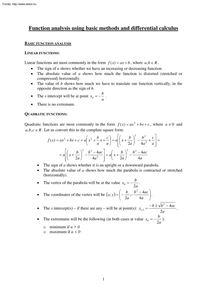
Function analysis using basic methods and differential calculus BASIC FUNCTION ANALYSIS LINEAR FUNCTIONS: Linear functions are most commonly in the form f ( x) = ax + b , where a, b ∈ R . • The sign of a shows whether we have an increasing or decreasing function. • The absolute value of a shows how much the function is distorted (stretched or compressed) horizontally. • The value of b shows how much we have to translate our function vertically, in the opposite direction as the sign of b. b • The x intercept will be at point x0 = − . a • There is no extremum. QUADRATIC FUNCTIONS: Quadratic functions are most commonly in the form f ( x) = ax 2 + bx + c , where a ≠ 0 and a, b, c ∈ R . Let us convert this to the complete square form: 2  c b  b2 c  2 b f ( x) = ax + bx + c = a x + x +  = a  x +  − 2 + = 2a  a a a  4a   2 2  b  b 2 − 4ac  b  b 2 − 4ac  − a x − = + = a  x +  

  2a  2a  4a 4a 2    The sign of a shows whether it is an upright or a downward parabola. The absolute value of a shows how much the parabola is contracted or stretched (horizontally). b The vertex of the parabola will be at the value x0 = − . 2a  b b 2 − 4ac  . The coordinates of the vertex will be (x; y ) =  − ;− 4a   2a 2 • • • • • • − b ± b 2 − 4ac The x intercept(s) – if there are any – will be at point(s): x1, 2 = . 2a b The extremums will be the following (in both cases at value x0 = − ): 2a o minimum if a > 0 o maximum if a < 0 1 VIEWPOINTS OF BASIC FUNCTION ANALYSIS: • • • Domain : Range: Monotonity: • • Zero values: Extremums: • Bounds: • Convexity: • Parity: • Periodicity: The set of all input values of a function. The set of all possible output values of a function. A function is monotonic increasing [decreasing] when for any x1 < x 2 it is true

that f ( x1 ) ≤ f ( x 2 ) [ f ( x1 ) ≥ f ( x 2 ) ]. A function is strictly monotonic increasing [decreasing] when for any x1 < x 2 it is true that f ( x1 ) < f ( x 2 ) [ f ( x1 ) > f ( x 2 ) ]. The values of the range, where f ( x) = 0 . The function has a minimum [maximum] at x1 [ x 2 ] if there is no smaller [greater] value of the range than f ( x1 ) [ f ( x 2 ) ]. A local extremum is an extremum within an interval, though this might coincide with the (global) extremum. A function is upper (lower) [or both] bounded if there exist a K number that f ( x) ≤ K ( f ( x) ≥ K ) [ f ( x) ≤ K ]. A function is convex if a segment connecting any two points of the function is above the function, else it is concave. A function is even if f (− x) = f ( x) , that is, it is symmetrical to the y axis. A function is odd if f (− x) = − f ( x) , that is, it is symmetrical to the origin. A function is periodical if there exists a p number that f ( x − p) = f ( x) = f ( x + p) .

FUNCTION TRANSFORMATIONS: Transformations of the function value: f ( x) + c The function is shifted upwards (if c > 0 ) or downwards (if c < 0 ) along the y axis by |c| units. The function is stretched (if c > 1 ) or compressed (if 0 < c < 1 ) along the y axis c ⋅ f (x) c-times. The function is reflected over the x axis. − f (x) Transformations of the variable: f ( x + c) The function is shifted left (if c > 0 ) or right (if c < 0 ) along the x axis by |c| units. f (c ⋅ x) The function is compressed (if c > 1 ) or stretched (if 0 < c < 1 ) along the x axis 1 -times. c The function is reflected over the y axis. f (− x) DIFFERENTIAL CALCULUS Differentiation expresses the rate at which a quantity (y) changes with respect to the change in another quantity (x), on which it has a functional relationship [that is, y is a function of x, and differentiation expresses the rate at which y changes in respect to the change in x]. 2 DEFINITIONS: def:

Differentia quotient: (also: Difference quotient) Let f be a real function with domain D f . Let x 0 be an inner point of the domain. The differentia quotient of function f at point x 0 is f ( x) − f ( x0 ) , where x ∈ D f {x0 } x − x0 [that is: the differentia (difference) quotient is the slope of the line connecting points ( x0 ; f ( x0 )) and ( x; f ( x)) ]. def: Differential quotient: If the finite real limit of the differentia quotient of function f in point x 0 exists [that is, function f can be differentiated in point x 0] the differential quotient of function f at point x 0 is f ( x) − f ( x0 ) lim x x0 x − x0 [that is: the differential quotient is the slope of the tangent drawn to function f at its point ( x0 ; f ( x0 )) ]. THEOREMS: 1) Continuity: Differentiability implies continuity, but not vice versa [that is, continuity is a necessary, but not sufficient condition of differentiability]. 2) Rules of differentiation: If functions f(x) and g(x) are differentiable

in point x 0 , then the following differential quotients exist in the same point, and the following relations are true: • • • • • (c ⋅ f )′ = c ⋅ f ′ , where c is a constant ( f ± g )′ = f ′ ± g ′ ( f ⋅ g )′ = f ′ ⋅ g + f ⋅ g ′ ′ f ( f ′ ⋅ g − f ⋅ g ′) , where g ( x ) ≠ 0   = 0 g2 g ( f  g )′ = ( f ′  g ) ⋅ g ′ [chain rule] 3) The derivative of some basic functions: • f ( x) = c • • • f ( x) = x f ( x) = a x f ( x) = e x • f ( x) = log a x • f ( x) = ln x n f ′( x) = 0 f ′( x) = nx n −1 • • f ( x) = sin x f ( x) = cos x f ′( x) = a x ln a f ′( x) = e x 1 1 f ′( x) = ln a x 1 f ′( x) = x • f ( x) = tan x • f ( x) = cot x 3 f ′( x) = cos x f ′( x) = − sin x 1 f ′( x) = cos 2 x 1 f ′( x) = − 2 sin x 4) Monotonity: If function f (x) can be differentiated on the interval [a; b] , and the derivative function of f (x) is positive

[negative] on this interval, then f (x) is strictly monotonic increasing [decreasing] on the interval. 5) Convexity: If function f (x) can be differentiated twice on the interval [a; b] , and the second derivative function of f (x) is positive [negative] on this interval, is convex then f (x) [concave] on the interval. 6) Extremum: If function f (x) can be differentiated on the interval [a; b] , and at point x 0 it has a local extremum then it is true that f ′( x0 ) = 0 (it is a necessary, but not sufficient condition). 7) Extremum: If function f (x) can be differentiated on the interval [a; b] , and at point x 0 f ′( x0 ) = 0 and the derivative changes signs then there is a local extremum of the function at point x 0 . 8) Theorem: The function f ( x) = x n (where n is a positive whole number) can be differentiated at all real values of x, and that will be: ( x n )′ = nx n −1 Proof (by means of total induction): • for n=1, it is true ( x ′ = 1 ) • Lets suppose that the

same is true for n, and let us show that it is true for n+1 as well. The condition of induction: ( x n )′ = nx n −1 • We know that x n +1 = x ⋅ x n , and by using the rule of product differentiation, we get: ( x ⋅ x n )′ = x ′ ⋅ x n + x ⋅ ( x n )′ = 1 ⋅ x n + x ⋅ n ⋅ x n −1 = (n + 1) ⋅ x n • We have proved the formula from n to n+1, thus it will be true for all positive whole power (in fact, it will be true for all real powers). 4 FUNCTION ANALYSIS USING DIFFERENTIAL CALCULUS 1. Let us differentiate function f (x) at least twice (thrice, if possible) thus we get f ′(x) , f ′′(x) and f ′′′(x) . 2. Let us find the zero values of f ′(x) and f ′′(x) 3. The function will be increasing on an interval if f ′( x) > 0 and decreasing if f ′( x) < 0 on the same interval. 4. The function will be convex (increasingly increasing or decreasing) on an interval if f ′′( x) > 0 and concave (decreasingly increasing or decreasing) if

f ′′( x) < 0 on the same interval. 5. The (local) extremums (minimums and maximums): the zero values of f ′(x) , such that they satisfy the sufficient conditions of an extremum [below]. 6. The inflection points: those zero values of f ′(x) that did not satisfy the sufficient conditions of an extremum, that is, are not extremums; and the zero values of f ′′(x) , such that they satisfy the sufficient conditions of an inflection point [below]. The necessary condition of an extremum: f ′( x) = 0 . The sufficient condition of an extremum: Function f ′(x) changes signs before and after its zero value, OR f ′′( x) ≠ 0 (minimum if f ′′( x) > 0 and maximum if f ′′( x) < 0 ). The necessary condition of an inflection point: f ′′( x) = 0 . The sufficient condition of an inflection point: Function f ′′(x) changes signs before and after its zero value, OR f ′′′( x) ≠ 0 . Note 1: A function may have an extremum at an inner point if it is not

differentiable at that given point. Note 2: A function may have an extremum at the endpoints of its domain if is an interval. APPLICATIONS OF DIFFERENTIAL CALCULUS 1. Physics (elaborated): • The velocity(time) function [ v(t ) ] is the first derivative of the displacement(time) function [ s (t ) ], where we differentiated by t. • The acceleration(time) function [ a(t ) ] is the first derivative of the velocity(time) function [ v(t ) ], thus the second derivative of the displacement(time) function [ s (t ) ], where we differentiated by t. • v(t ) = s ′(t ) , and also a(t ) = v ′(t ) = s ′′(t ) . 2. Economics: The Marginal Utility function is the first derivative of the Total Utility function. The flexibility of functions (how much does a function change in respective to the change of one [or more] of its components). 3. Error calculus (in sciences) 4. (Math problems regarding differentiation, for example function plotting, finding extremums, inflection points and the

tangent of a function.) 5