Fizika | Tanulmányok, esszék » Navigation for Autonomous Surface Vessels

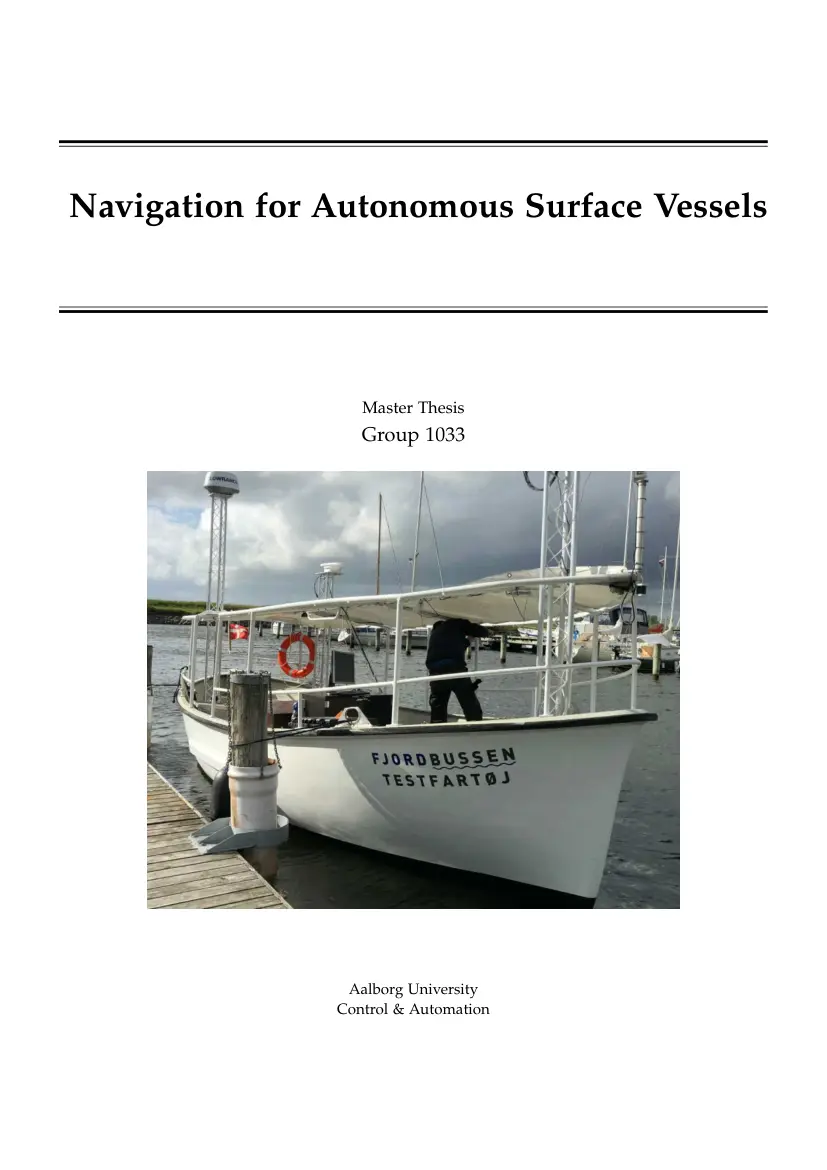
Navigation for Autonomous Surface Vessels Master Thesis Group 1033 Aalborg University Control & Automation Department of Automation & Control Control & Automation Fredrik Bajers Vej 7B DK-9000 Aalborg www.esaaudk Title: Navigation for Autonomous Surface Vessels Theme: Master Thesis Semester: 4th semester Control & Automation (MSc) Project Period: Spring semester 2020 Project Group: CA10-1033 Group Members: Mohamed Yahya Maad Simon Kaihøj Supervisors: Jesper Abildgaard Larsen jal@es.aaudk Report: 72 pages Submitted: June 4, 2020 Abstract: This thesis covers derivation of a non-linear model, simulation of this model, development of control systems and path planning systems for an Autonomous Surface Vessel. A nonlinear dynamic model was created using Newtonian mechanics in combination with hydrostatics. This model was implemented in both Simulink and Gazebo A PID controller was implemented, and the possibility of applying LPV control was investigated. The Artificial

Potential Field method and the State Lattice method were both implemented. Measurements made on the model were used to ensure that the State lattice was restricted to only finding paths that the system is capable of following. Preface This report documents the Master Thesis work carried out as part of the study program in Control & Automation at Aalborg University. The work is carried out as of an effort headed by ’Center for Logistik og Samarbejde’, aiming to create an autonomous ferry connection across the Limfjord in Aalborg, Denmark. The purpose of this thesis is to evaluate the feasibility of some of the methods and technologies considered to be used in the project, specifically within the areas of modeling, control, and path planning. To understand this thesis, it is beneficial to have fundamental knowledge of linear algebra, calculus and vector calculus. An understanding of basic control theory will also make some parts easier to understand. A familiarity with some

common methods used in path planning will aid in understanding of the proposed motion planners. References are made using the IEEE referencing scheme. Numbers in square brackets [1] refer to an entry in the bibliography Equations are referred to by the equation identifier in a parenthesis, so (1,2) would refer to the second equation in the first chapter. The thesis is written in the hope that it can serve as a reference for future students and researchers working on Autonomous Surface Vessels. The report’s structure is built up from seven chapters, each covering a significant part of the entire project. Chapter 1 introduces the problem, and introduces the architecture into which the components developed in this report fits. Chapter 2 describes how modeling of marine crafts is done, and derives the model of the vessel and its parameters. The chapter concludes with a symbolic structure of the equations of motion describing the system. Chapter 3 describes how the model was implemented

in both Gazebo and Simulink. Chapter 4 proposes two different methods for designing a controller capable of controlling the vessel. It also includes some analysis of why an one linearization strategy does not work. ii Chapter 5 lays out two different path planning strategies, the Artificial Potential Field method and the State Lattice method. It also describes how to generate a set of motion primitives for use with the State Lattice method. Chapter 6 shows the results from the different chapters. Chapter 7 presents the conclusions that can be drawn from the project, as well as what future work could be done to improve the project. Aalborg University, July 4, 2020 Mohamed Yahya Maad Simon Kaihøj mmaad18@student.aaudk skaiha@student.aaudk iii Acknowledgements Thanks Jesper :) Thanks Tor Einar Berg et al. iv Contents 1 Introduction 1 2 System Modelling 4 2.1 Basic Ship Theory . 4 Slicing Planes . 5 Lines

Plan . 6 Moulded Dimensions . 7 Coefficients of Form . 7 Metacentric Height . 9 2.2 Reference Frames and Coordinate Systems . 10 2.3 Forces and Torques, Mechanical . 12 Added Mass Matrix . 13 Coreolis-centripetal Matrix . 14 Heave Hydrostatic Force . 14 Buoyancy Forces and Torques . 15 Ballast Forces and Torques . 16 Propeller Forces and Torques . 16 Damping Forces and Torques . 17 Forces and Torques, Environmental . 17 Wind Forces and Torques . 17 Finding wind coefficients, Blendermann . 19 Wave Forces and Torques . 19 BODY to NED transformation . 19 NED to ENU

transformation . 21 2.4 2.5 v 3 Simulation 3.1 3.2 22 Simulink Simulation . 22 Buoyancy Simulation . 22 Mass and Coreolis Simulation . 23 Wind Simulation . 23 Drag Simulation . 25 Thrust Simulation . 25 Dynamic Model Base . 26 Gazebo Simulation . 26 4 Controller Design 4.1 30 Trolley Steering Method . 30 The Concept . 30 Steering Error Calculation . 31 4.2 PID Control . 32 4.3 Linear Parameter Dependent Plant . 35 Example Showing That Jacobian Linearization Does Not Always Work . 37 Linear Parameter Varying Control . 38 Stability Notions for LPV

Systems . 39 Generic Parameter Dependent Systems . 40 Quadratic Stabilization by State-Feedback, Generic LPV . 42 4.4 Quadratic Stabilization by Dynamic-Output Feedback, Generic LPV 42 Polytopic LPV Systems . 44 Quadratic Stabilization by State-Feedback, Polytopic LPV . 44 LPV Systems in LFT Form . 45 5 Motion Planning 47 5.1 Artificial Potential Fields . 47 5.2 State-lattice . 49 Motion Primitives . 53 vi 6 Results 59 6.1 Simulation Verification . 59 Max thrust forward . 59 Set Zig-Zag Maneuver for comparison . 60 PID Controller Results . 62 PID Zig-Zag Maneuver . 63 PID Circle Maneuver . 63 6.3 Model Analysis .

64 6.4 Motion Planning Results . 65 6.2 7 Evaluation 68 7.1 Conclusion . 68 7.2 Future Work . 68 Modeling . 68 Simulation . 69 Control . 69 Motion Planning . 69 Bibliography 70 A Gazebo Code 72 vii CHAPTER | 1 Introduction The cities of Aalborg and Nørresundby, Denmark, both being part of the same metropolitan area, are divided by a body of water, with the main city centre (Aalborg) located on the south side. There exists 3 connections between the north and the south within the cities, one highway tunnel, one bridge for cars, pedestrians and bicyclists, and one bridge for trains, pedestrians and bicyclists. Both of the bridges are in the western end of the city, and there exists an area underserved by public transport in the north east. This

area is scheduled to be developed into housing, and a connection from there to the south bank would help alleviate the need for a large degree of personal motor vehicle ownership. Fig. 11 The existing ways to cross the water, along with the proposed new route. The municipal government has decided to explore the possibility of an autonomous surface vessel ferrying passengers/bicyclists across the water, mainly to increase the access from this new housing development to the city centre, and vice versa. The first planned route is 500-600m long, depending on the exact choice of the locations and size of the piers. The route never takes the vessel far from shore, and as such, if the weather starts worsening to the point beyond the capabilities of the vessel, it can simply dock 1 Introduction and wait for the weather to improve. This is in contrast to an oceangoing vessel that must be able to handle any weather that is reasonably possible to occur on any given voyage, or risk loss of

life. The vessel discussed in this project still needs to be able to handle the weather most days, as this is one of the most important considerations for uptime. In the plan laid out by the municipal government, there would be a manned control room on shore, for monitoring the autonomous vessels, and raising the alarm if anything goes wrong. This control room would be managing multiple vessels at once, and would not necessarily be located physically close to the water to launch a rescue operation. Approximately every 5 years an event known as The Tall Ship Races comes to the city, resulting in lots of traffic on the water for a week. Outside of this and similar events, there is only sparse traffic on the water. It has therefore been decided that the autonomy system does not need to handle the heavy traffic during these events, instead the boats would be manned and manually controlled during these times. This project was initially intended to include development and testing of a

physical test vessel, but because of events beyond the control of the project group, this was cancelled. Instead this project will consider the Research vessel RV Gunnerus, because a large amount of data about its physical properties are available, meaning that a decent model can be made. RV Gunnerus is a research vessel owned and operated by the Norwegian university NTNU. How can a vessel be made to autonomously sail back and forth ferrying passengers on the given route? For this there must be a vessel that can be controlled autonomously (as in, the controls of the vessel can be actuated by another system, not a human), an autonomy system, encompassing navigation, control, and other computational tasks, and lastly a sensing system, for positioning and obstacle detection. This paper focuses on the autonomy system but may discuss the others to the extent they affect the former. The vessel itself can be made in one of two ways. Either an existing vessel can be modified to accept inputs

from the autonomy system, such as by mounting servomotors on the controls. Otherwise a ship purposefully built for autonomous control can be used. Other intermediate options exit, such as for vessels that are made with an autopilot system which can be replaced. The sensor system consists of all the sensors that can function as inputs to the autonomy system. These fall broadly into two categories, those sensing information about the state of the vessel, and those that sense the surroundings Measuring the state of the vessel could include such things as gyroscopes for measuring the angular velocity, accelerometers for measuring acceleration, magnetometers 2 Introduction for measuring compass heading, GPS systems for measuring position and velocity, anemometers for measuring relative wind speed and direction, and logs for measuring the speed through the water. These sensors would mainly be used by the control system, but would also inform the navigation system on where to navigate from.

The sensors for sensing the world around the vessel could include such things as radar, lidar, and cameras with obstacle detection algorithms, and might also include AIS transponders to include information sent by other vessels operating in the same area. These sensors would not directly influence the controller, but instead, their data would be used by the navigation subsystem to determine where there are obstacles to be avoided. The autonomy system discussed in this paper would mainly consist of two parts; the navigation subsystem and the control subsystem. The navigation system is responsible for plotting a course that will get the vessel from the current position to the goal position, without colliding with obstacles, while the control system is responsible for following this path. A controller is a system for generating the inputs to a plan (in this case the plant is an autonomous surface vessel), such that the state of the system reaches a desired state. Therefore, to make a

controller it is beneficial to have a model that describes how the plant reacts to any inputs the controller may generate. The next chapter will describe how to make such a model. 3 CHAPTER | 2 System Modelling The whole goal of this chapter is to find a complete dynamic model for any water vehicle, and to prove how a dynamic model of the form 2.1 is derived, which is the dynamic model of a vehicle in the BODY reference frame. This can later be transformed to other reference frames as desired [2]. M ν̇ + C (ν)ν + D (ν)ν + g(η ) + g0 = τ + τwind + τwave (2.1) With a complete dynamic model an advanced simulation environment can be created, enabling development of control strategies in a cost-efficient and safe environment, while also allowing “auto-tuning” by tools such as the MatLAB MPCtoolbox. The table below introduces variables used to describe forces, positions and velocities of a boat. These will be used throughout this chapter Direction Force Position

Velocity Linear along x-axis (surge) X x u Linear along y-axis (sway) Y y v Linear along z-axis (heave) Z z w Angular about x-axis (roll, heel) K φ p Angular about y-axis (pitch, trim) M θ q Angular about z-axis (yaw) N ψ r 2.1 Basic Ship Theory To be able to understand the data sheets and dimensions describing a boat, such as the one in figure 2.1, some basic ship theory must be introduced These dimensions will later be used as constants in the dynamic model of the boat. It was also an option to approximate the behaviour of the boat using some of these dimensions in the same way as in [3], [4] or [5]. That was omitted either due to verification difficulties, lack of detailed hull data, or unavailable software packages. 4 System Modelling Fig. 21 2.1 Basic Ship Theory Some technical data about the RV Gunnerus [6] Slicing Planes The dimensions of a boat can be described by a set of planes slicing through its’ hull. As seen in figure 22, three types

of planes exist: The middle line plane, which is, more often than not, the boats’ only plane of symmetry. The shape created by a cut using the middle line plane is also called the sheer profile or plan. The design waterplane goes along the plane which would separate a boat into two parts, one part in the water and one in the air, when the boat stands still and there are no waves. All planes parallel to the design waterplane are called waterplanes The planes which are perpendicular to both the middle line plane and the waterplanes, are called transverse planes. 5 System Modelling Fig. 22 2.1 Basic Ship Theory Figure illustrating the different planes the vessel can be segmented along [7]. As seen in figure 2.3, the point between AP and FP is called the (a)midship, which is also a transverse plane. AP, or after perpendicular, is the line defining where the rudders are. FP, or fore perpendicular, is where the design waterplane and stem of the ship intersect. Midship is often

denoted by the symbol: ⊗ , where the cross exceeds the circle. Depending on the ship, there will often be around 20 transverse planes with equal distance between FP and AP, to achieve the proper decimation [7]. Fig. 23 This shows the location of AP, FP, LOA , and midships, among other important points and measurements. [8] Lines Plan Figure 2.4 contains the whole lines plan, including the sheer, body and half breadth plan. A lines plan describes the shapes of the hull by showing the contour of the 6 System Modelling 2.1 Basic Ship Theory hull on different planes. The lower part of figure 24 illustrates the half breadth plan, where the contour of the hull is shown when sliced by different waterplanes. At the points where transverse planes and this contour intersects, a distance y is defined. The different values of y can be compiled into a table of offsets A table of offsets is used to describe the shape of the hull, such that it can be imported into digital design or analysis

tools, such as MultiSurf or ShipX VERES. These can then be used to find and simulate the behaviour of the ship. As no table of offsets was available, no such tools is being used. Fig. 24 The lines plan shows the Body plan, Sheer plan and Half breadth plan [7] Moulded Dimensions In figure 2.5 a differentiation between the inner and outer surface of the hull is presented. The displacement dimensions are defined as the dimensions wetted by the sea. The displacement line goes along the outside of hull, separating hull from water Meanwhile, the moulded line, or moulded dimensions, is defined as the displacement line minus hull thickness, resulting in a line describing the inside of the hull of a ship. It is important to notice this difference when reading datasheets, as some define the data of ships in moulded dimensions, while others do not. The moulded depth of the ship D is separated into two parts: the moulded draught T and freeboard f , as seen in figure 2.6 On top of that comes the

height difference caused by camber, which helps water flow off the deck. Coefficients of Form When examining the hydrodynamic properties of a ship, some coefficients may be used to classify the relationship between the hull and the behaviour of the ship, namely the coefficients of form. Ships with similar coefficients should have relatively similar behaviour. These coefficients may be used for ship behaviour approximation The dimensions in figure 27 are essential when finding the coefficients of form. 7 System Modelling 2.1 Basic Ship Theory Fig. 25 hull The difference between the moulded line and the displacement line is the thickness of the Fig. 26 The moulded depth can be contrasted with the moulded draught and the freeboard [8]. ∇ is the volume of displacement, describing the amount of fluid displaced by the ship. CWP is the coefficient of fineness of water, which describes the ratio between the area of a waterplane AW and the area of the box around it made by LW L B.

CWP = AW LW L B (2.2) CM is the midship coefficient, which describes the ratio between the area of the submerged transverse plane amidship A M and the area of the box around it made by BT. 8 System Modelling 2.1 Basic Ship Theory Fig. 27 Figure showing the area of the planes AW and A M , in addition to some other basic dimensions to find the coefficients of form CM = AM BT (2.3) CB is the block coefficient, which describes the ratio between the volume of displacement ∇ and the volume of the block around it made by BTL pp . CB = ∇ BTL pp (2.4) CP is the longitudinal prismatic coefficient, which describes the ratio between the volume of displacement ∇ and the volume of the prism around it made by A M L pp . CP = ∇ A M L pp (2.5) CVP is the vertical prismatic coefficient, which describes the ratio between the volume of displacement ∇ and the volume of the prism around it made by AW T CVP = ∇ AW T (2.6) Metacentric Height To describe the metacentric height,

the floating box illustrated in figure 2.8 is used For convenience of illustration, imagine the waterline is being rotated instead of the box. When the box is at an equilibrium, the waterline will go along the dashed line, and the center of buoyancy will be at point B. If the box/waterline is to be rotated with an angle φ, the new center of buoyancy will be at point B1 . Lines which are perpendicular to the waterline and going through B or B1 can then be created. The intersection between these new lines is called the metacentre, denoted 9 System Modelling 2.2 Reference Frames and Coordinate Systems as the point MT , where the T stands for transverse as this case is for the rotation about the x-axis of the ship. The transverse metacentric height GM T is therefore the distance between the center of gravity, here denoted as the point G, and the metacentre MT . The same procedure should be followed when finding the transverse metacentric height GM L , but rotate an angle θ about the

y-axis of the boat. More about the axis system of a boat can be found in figure 2.10 Fig. 28 Figure illustrating the concept of metacentric height Notice that this is in the NED reference frame, hence positive z is downwards [2]. 2.2 Reference Frames and Coordinate Systems Different reference frames are used as some calculations are easier done in some frames than others. Four reference frames are looked into in this project: • ECI := {i} ∼ Earth-centered inertial frame • ECEF := {e} ∼ Earth-centered Earth-fixed reference frame • NED := {n} ∼ North-East-Down • BODY := {b} ∼ Body-fixed reference frame The following vector notation is used to express how positions and velocities are defined wrt. the different reference frames: un := ~u in {n}. 10 System Modelling Fig. 29 2.2 Reference Frames and Coordinate Systems Figure showing the NED coordinate system [9]. n u = h u1n u2n u3n iT (2.7) veb/n := Linear velocity of ob wrt. {n} expressed in {e} b ωn/e :=

Angular velocity of {n} wrt. {e} expressed in {b} θnb := Euler angle between {n} and {b}. The standard way of rotating something within a reference frame, is to use rotation matrices: Rotation about x-axis:   0 0  1   R x (θ ) = 0 cos θ − sin θ    0 sin θ cos θ (2.8) Rotation about y-axis:    cos θ 0 sin θ    Ry (θ ) =  0 1 0    − sin θ 0 cos θ 11 (2.9) System Modelling 2.3 Forces and Torques, Mechanical Rotation about z-axis:   cos θ − sin θ 0     Rz (θ ) =  sin θ cos θ 0   0 0 1 (2.10) These matrices will later be used to calculate forces when rotated, or transforming them from one coordinate system to another. Certain important points on a boat needs to be defined, as the distances between them are used to calculate torques on the body of the ship. These points are shown on figure 2.10 • CG ∼ Center of gravity. • CB ∼ Center of buoyancy. • CF ∼

Center of flotation. • CO ∼ Center of origin. Fig. 210 Figure showing some central points on a boat Most important are center of gravity (CG) and center of buoyancy (CB) [2]. One of these distances is the vector ~r g , which is the vector between CO and CG in {b}. This is used to calculate the rigid-body added mass and coreolis matrices in the next section. 2.3 Forces and Torques, Mechanical This section explains how forces and torques are found, excluding forces from wind and waves, hence the section title. 12 System Modelling 2.3 Forces and Torques, Mechanical The matrix cross product operator is defined as: λ × a := S(λ) a (2.11) h iT λ = λ1 λ2 λ3 (2.12) where: and:   − λ3 λ2   0   S ( λ ) = − S ( λ ) =  λ3 0 − λ1    − λ2 λ1 0 T (2.13) This will be used when calculating the added mass and coreolis-centripetal matrices. It should also be noted that the vector ν is a combination of linear and angular

velocities in {b}. ν1 represents the linear velocities (u, v, w), and ν2 the angular velocities ( p, q, r ):   h iT ν1 ν= = u v w p q r ν2 (2.14) Added Mass Matrix Added mass is a concept which describes the mass distribution within an object, represented as a matrix. The added mass may be separated into two parts, the rigid body inertia matrix MRB and the hydrodynamic inertia matrix M A . M = MRB + M A (2.15) MRB is defined as:  MRB =  mI3×3 mS(r bg )  −mS(r bg )  I0 (2.16) Where I0 is the inertia matrix. M A on the other hand has to be identified, either by performing frequency-response tests on the boat, or by using simulation software where the hull of the boat is imported and analyzed. 13 System Modelling 2.3 Forces and Torques, Mechanical Coreolis-centripetal Matrix The coreolis-centripetal forces may also be separated into two parts, the rigid body matrix CRB (ν) and the hydrodynamic matrix C A (ν). C = CRB + C A (2.17) CRB (ν)

is defined as:  CRB =  03 × 3 −mS(ν1 ) − mS(ν2 )S(r bg )  −mS(ν1 ) + mS(r bg )S(ν2 ) −S( Ib ν2 )  (2.18) Where Ib is the inertia matrix of the hull of the boat. C A (ν) is dependent on the hydrodynamic inertia matrix M A , where M A is divided into four 3 × 3 matrices:  MA =  A11 A12 A21 A22  (2.19)  C A (ν) is then defined as:  C A (ν) =  −S( A11 ν1 + A12 ν2 ) 03 × 3 −S( A11 ν1 + A12 ν2 ) −S( A21 ν1 + A22 ν2 )   (2.20) Heave Hydrostatic Force The nabla symbol ∇ is used to indicate the static water displacement of the boat, while δ∇(z) is the change of water displacement depending on the height of the boat z with respect to the design waterplane. The force Z is the difference between gravitational and buoyancy forces. δ∇(z) is defined as: δ∇(z) = Z z 0 Awp (ζ )dζ (2.21) Where Awp (ζ ) is a function returning the area of the waterplane depending on the displacement height z. If the

shape of the hull and the height of the design waterplane allows it, δ∇(z) can be approximated to a linear function. This will have the following form, where one needs to know the height ζ and area of a waterplane Awp (ζ ), at two points: 14 System Modelling 2.3 Forces and Torques, Mechanical a is the slope of the linear function: a= Awp (ζ 2 ) − Awp (ζ 1 ) ζ1 − ζ2 (2.22) A new waterplane at height z can then defined as: Awp (z) = Awp (ζ 1 ) + a(ζ 1 − z) (2.23) Integrating equation 2.23 from 0 to z results in the difference in volume due to variation of height from design waterline to z: 1 δ∇(z) = Awp (ζ 1 )z + aζ 1 z + az2 2 (2.24) The force Z is defined as: Z = mg − ρg(∇ + δ∇(z)) = −ρgδ∇(z) (2.25) When a boat is in steady-state, the buoyancy force cancels out the gravitational force, so both Z and z are zero. Fig. 211 z. [2] Figure illustrating the change in submerged volume of a box caused by change in height Buoyancy Forces and

Torques The buoyancy forces are dependent on the heave force Z, while the torques depend on the transverse and longitudinal metacentric heigts, GM T and GM L . The vector g(η ) contains the buoyancy forces and torques, and is defined as: 15 System Modelling 2.3 Forces and Torques, Mechanical        g(η ) = ρg       Rz − 0 Awp (ζ )dζ sin θ Rz Awp (ζ )dζ cos θ sin φ 0 Rz 0 Awp (ζ )dζ cos θ cos φ ∇ GM T sin φ cos θ cos φ ∇ GM L sin θ cos θ cos φ ∇(− GM L cos θ + GM T ) sin φ sin θ              (2.26) Ballast Forces and Torques The ballast forces and torques are embedded into g0 , which is defined as:   0     0      − ∑n V   i =1 i  g0 = ρg   − ∑n yi Vi  i = 1    n   ∑i=1 xi Vi    0 (2.27) Where i signifies each ballast tank, while xi and yi is the x-y positions of a given

ballast tank. Vi is the volume of the water in that tank n represents the number of ballast tanks. Propeller Forces and Torques The propulsion system is modelled as a collection of azimuth thrusters. This was done to replicate the propulsion system of R/V Gunnerus. Each propeller has a thrust magnitude f , and a turning angle α. The generalized force F is then defined as:    f cos α   F =  f sin α    0 (2.28) T is the generalized torque produced by a propeller: T =r×F 16 (2.29) System Modelling 2.4 Forces and Torques, Environmental Where r is the vector from CG to the center of thrust. The forces and torques are embedded into the vector τ, which is defined as:   F τ=  T (2.30) Damping Forces and Torques The damping forces/torques can be separated into two parts, a linear and nonlinear part, as presented in the following equation: D (νr ) = D + Dn (νr ) (2.31) Where νr is the difference between the boats’ linear

velocities ν and water current velocities νc . Both are represented in BODY coordinates h iT νc = uc vc wc 0 0 0 (2.32) νr = ν − νc (2.33) Both damping matrices have to be determined either by measurements or using by suitable software, such as VERES. The simulation of memory effect was omitted due to lack of available empirical data. 2.4 Forces and Torques, Environmental This section explains how environmental forces and torques are calculated. Wind Forces and Torques When measuring the angle of the wind β w , forward is always along xb . This is most likely how an onboard anemometer would report the angle as well. The wind speed Vw can be decomposed into uw and vw . uw = Vw cos( β w − ψ) (2.34) vw = Vw sin( β w − ψ) (2.35) These will be used to find the relative velocities urw and vrw : 17 System Modelling 2.4 Forces and Torques, Environmental urw = u − uw (2.36) vrw = v − vw (2.37) This can then be used to calculate the relative wind speed

and angle of attack, Vrw and γrw : Vrw = q u2rw + v2rw (2.38) γrw = − arctan(vrw , urw ) (2.39) The forces and torques from the wind are then defined as:    CX (γrw ) A Fw     CY (γrw ) A Lw     C (γ ) A  1 rw Z Fw   2 τwind = ρ a Vrw    CK (γrw ) A Lw HLw  2     CM (γrw ) A Fw HFw    CN (γrw ) A Lw Loa (2.40) Where: • Ci := Wind coefficients, found either by measurements, software or lookuptables • ρ a := Air density • A Fw := Frontal projected area • A Lw := Lateral projected area • HFw := Centroid of A Fw above water line • HLw := Centroid of A Lw above water line • Loa := Overall length 18 System Modelling 2.5 BODY to NED transformation Finding wind coefficients, Blendermann One way of finding the wind coefficients of a ship is by using the estimations of Blendermann, where four parameters are used to characterize a ship: Transverse resistance CDt , longitudinal

resistance CDl , cross-force parameter δ and rolling moment factor κ. The longitudinal resistance CDl is found using the longitudinal resistance coefficient CDl AF which is estimated by Blendermann. CDl = CDl AF (γw ) A Fw A Lw (2.41) The wind coefficients are found in the following equations: CX (γw ) = −CDl A Lw A Fw CY (γw ) = CDt cos(γw ) δ CDl 1 − (1 − ) sin2 (2(γw )) 2 CDt sin(γw ) δ CDl 1 − (1 − ) sin2 (2(γw )) 2 CDt CK (γw ) = κCY (γw ) C N ( γw ) = [ sL π − 0.18(γw − )]CY (γw ) Loa 2 (2.42) (2.43) (2.44) (2.45) Where s L is the centroid of A Lw . Wave Forces and Torques The wave forces and torques were not implemented due to the lack of Response Amplitude Operators for the R/V Gunnerus. 2.5 BODY to NED transformation When working with a simulation environment using the NED coordinate system, a transformation of the dynamic model from BODY to NED is needed. h i Θnb = φ θ ψ (2.46) Using a ZYX-rotation matrix gives the

following rotation matrix: Rnb (Θnb ) := Rz (ψ) Ry (θ ) R x (φ) 19 (2.47) System Modelling Fig. 212 2.5 BODY to NED transformation Table showing the wind coefficient parameters estimated by Blendermann [10]. The matrix TΘ (Θnb ) is defined as:  1 sin φ tan θ cos φ tan θ   TΘ (Θnb ) = 0  0   − sin φ   cos φ  cos θ cos φ sin φ cos θ (2.48) The matrix JΘ (η ) is the transformation matrix used to transform forces and vectors from {b} to {n} coordinate systems.  JΘ (η ) :=  Rnb (Θnb ) 03×3 03 × 3 TΘ (Θnb ) T  (2.49) h iT η := N E D φ θ ψ (2.50) η̇ = JΘ (η )ν (2.51) η̈ = JΘ (η )ν̇ + J̇Θ (η )ν (2.52) Where η is defined as: All variables with a star ∗ are in the NED coordinate system: 20 System Modelling 2.5 BODY to NED transformation Added mass matrix: −T M∗ (η ) = JΘ (η ) MJΘ−1 (η ) (2.53) −T C ∗ (ν, η ) = JΘ (η )[C (ν) − MJΘ−1 (η ) J̇Θ

(η )] JΘ−1 (η ) (2.54) −T D ∗ (ν, η ) = JΘ (η ) D (ν) JΘ−1 (η ) (2.55) Coreolis matrix: Damping matrix: Forces and torques caused by buoyancy and ballast: −T g∗ (η ) + g0∗ = JΘ ( g ( η ) + g0 ) (2.56) Forces and torques from propulsion system, wind and waves: ∗ ∗ τ ∗ + τwind = JΘ−T (τ + τwind + τwave ) + τwave (2.57) When combined, this results in a transformed dynamic model in NED: ∗ ∗ η̈ = M∗ (η )−1 (−C ∗ (ν, η )η̇ − D ∗ (ν, η )η̇ − g∗ (η ) − g0∗ + τ ∗ + τwind + τwave ) (2.58) Both the simulation environments in Simulink and Gazebo are based on equation 2.58, but as shown in the following subsection, the NED coordinates are transformed to ENU for better visualization In the following chapter a detailed explanation of the simulation environments will be presented. NED to ENU transformation The ENU positions is used for looking at the simulation results in Simulink, and is the general

coordinate system used in Gazebo.  ENU =  R x (φ) 03 × 3 03×3 R x (φ) 21  η (2.59) CHAPTER | 3 Simulation When tuning and testing controllers, either the real system which is to be controlled or a simulation of it may be used. Accurate simulations have the advantage of producing similar results, while removing the cost of operating and performing tests on the real system. It also speeds up efficiency, where different tests may run in parallel, and removes inaccessibility problems. This chapter explains in detail simulations made in two environments, Simulink and Gazebo [11]. Simulink is used to iron out model errors, while Gazebo is used for better visualization and in combination with ROS to emulate interaction with hardware. All underlying code is based on the theory of chapter 2, and the code itself can be found in appendix A. 3.1 Simulink Simulation This section will be used to explain the structure of the Simulink simulation. As seen in figure 3.1 the

blocks are colour-coded to help show which blocks belong in the same category. The system as a whole has two inputs: The propeller force f and angle α to the teal thrust calculation block, and one output: The ENU position from the rightmost white block, the NED to ENU transformation block. The small white blocks are parameters which are generated in their own MatLAB script, making it easier to keep track of the values of the parameters. Buoyancy Simulation The blocks shown in figure 3.2 are based on subsections Heave Hydrostatic Force and Buoyancy in section 2.3, and are used to calculate the total buoyancy forces and torques. The change of submerged hull volume with regards to change in height z is first calculated in “IAWP”. This is then sent to “BUOYANCY”, which calculates the buoyancy forces and torques. The block named “BALLAST” calculates the change in buoyancy caused by ballast tanks. 22 Simulation 3.1 Simulink Simulation Fig. 31 Figure showing an overview of

the whole simulation setup in simulink The blocks are color-coded to show which ones belong together. “VI”, “XI” and “YI” are vectors containing the information about the volume, xposition and y-position of each ballast tank. Mass and Coreolis Simulation The blocks shown in figure 3.3 are based on subsections Added Mass and Coreolis in section 2.3, and are used to calculate the added mass and coreolis matrices The body velocities denoted as “v” come from the dynamic model, representing the vector ν. The variable “RGB” contains the vector r bg . Wind Simulation The blocks shown in figure 3.4 are based on subsections Wind Forces and Torques and Finding wind coefficients, Blendermann in section 2.4, and are used to calculate the forces and torques applied on the boat by the wind 23 Simulation 3.1 Simulink Simulation Fig. 32 Fig. 33 Figure showing the blocks simulating hydrostatic forces. Figure illustrating the blocks which generate the added mass and

coreolis matrices. The relative wind speed Vrw and angle γrw are first calculated in “WINDGAMRW”. The angle is then sent to “COFGAM”, which calculates the corresponding wind coefficient. The block “WIND” uses the wind speed and coefficient from the previous blocks to calculate the wind forces and torques. 24 Simulation Fig. 34 3.1 Simulink Simulation Figure showing the blocks which generate forces applied on the boat by wind. Drag Simulation The block shown in figure 3.5 is based on the subsection Damping Forces and Torques in section 2.3, and is used to calculate the forces and torques created by the drag and damping from the water. v is the velocities of the boat ν, while Vc is the velocities of the current νc . Fig. 35 Figure showing the block which calculates drag. DL is the linear drag term Thrust Simulation The block shown in figure 3.6 is based on the subsection Propeller Forces and Torques in section 2.3, and is used to calculate the forces and torques

generated by the azimuth thrusters. This is the only block which receives control signals. 25 Simulation Fig. 36 3.2 Gazebo Simulation Figure showing the block which calculates the force produced by the azimuth thruster. Dynamic Model Base The block shown in figure 3.6 is based on section 25, and is used to ultimately find the systems positions in an ENU reference frame. As some of the produced forces and torques are dependent on the velocities in {b}, ν, and the positions in {n}, η, they are first calculated in the blocks presented in the previous subsections, which feed the results into “VD” and “ETADD”. The blocks “VD” and “ETADD” are semi-independent of each other, as they are not directly connected in any way. The block “JMATRIX” is used to calculate the matrix JΘ (η ). After finding η, “NED2GLOBAL” is used to transform the positions from the NED to ENU reference frame. This is the only block with an output going out of the overall system. 3.2

Gazebo Simulation The Gazebo simulation plug-in is based on the Simulink setup presented in section 3.1 The code has the same modular structure, made with a class hierarchy which allows for changes to be made without having modify the main logic of the plug-in. The plug-in is separated into three parts: The world file which binds all necessary information together. While it is possible to write logic for objects in this file, only code for world settings like gravity is written. It does point to the C++ code, which contains all the logic for the boat, and it points to the model of the boat, which can be seen in figure 3.8 The C++ code contains all the logic for the boat, including a rudder which shows the direction of the rear thrusters. For visual representation, a model of a RIB and a rudder are made in Blender to be imported into Gazebo. These models do not contain any kind of logic, except for collision boundaries. 26 Simulation Fig. 37 3.2 Gazebo Simulation Figure showing

the blocks which calculate the states in BODY and NED reference frames. Fig. 38 Figure showing a small boat with a rudder, representing Gunnerus and the angle of the azimuth thruster. Each part of the dynamic model is segregated into separate C++ files, with a class hierarchy as shown in figure 3.9 R/V Gunnerus does have a bow thruster, which is not modelled in Simulink or included in the C++ code, since the bow thruster is deemed unnecessary as this thesis does not tackle the problem of docking. If it is 27 Simulation 3.2 Gazebo Simulation ever needed in the future, any thrusters can easily be added due to the modular code structure. All constants are in the main file “BoatCode.cc” 28 Simulation Fig. 39 3.2 Gazebo Simulation Figure showing a class diagram of the implementation in Gazebo. 29 CHAPTER | 4 Controller Design This chapter presents the design paradigms for two controllers, the PID and the LPV controller. The PID controller is a classical controller with

no predictive capabilities. The input is often the difference between reference and output feedback. In this case the error is a turning angle error calculated by the trolley steering method. PID controllers were originally designed for automatic ship control in 1922, by observation of the helmsman at ships. This in itself was motivation for using the PID controller as a benchmark. A Linear Parameter Varying (LPV) controller is a state-space controller with predictive capabilities due to the LPV model. The input can either be state-feedback or output feedback. In the case of output feedback, and LPV model will be part of an observer which can estimate the states of the real system. If certain conditions are met, an LPV controller may have guarantees for stability The motivation for using an LPV controller is the need for a nonlinear controller with prediction capabilities, and which can handle a MIMO system. 4.1 Trolley Steering Method Since boats can drift, and the heading of a

boat does not equal the direction it is moving, the controller needs a corrected error signal. One way to solve this is by using the trolley steering method, which will be explained in this section. The Concept The concept of this method is derived from the behaviour of a trolley with a handlebar. The steering of the trolley is determined by the handlebar, which controls the wheels, as seen 4.1 This concept can be transformed for use with autonomous planar vehicles, with a virtual handlebar which points towards a point on a path which is to be followed. The handlebar controls the steering mechanism of the vehicle, and the length of the handlebar decides how aggressively the vehicle will react to change of direction caused by the points on the path. A longer handle means smaller steering angles, as will be explained in the coming subsection [12]. 30 Controller Design 4.1 Trolley Steering Method Fig. 41 Figure showing a trolley and a handlebar [12]. Steering Error Calculation When

a path is generated, it comes in the format of array of points. In this thesis a distance of 10 cm is selected as the maximum distance between each point. The setup for the trolley steering method with a boat is illustrated in figure 4.2 For the trolley steering method to work, an origin ( x0 , y0 ) for the virtual handlebar must first be decided. A search space is then defined, with a minimum and a maximum distance, dmin and dmax , from ( x0 , y0 ). In this search space, the first point to be found along the path with a distance ∈ [dmin , dmax ], is selected to be the end of the handlebar ( x p , y p ). The distance d is calculated by the following equation: d= q ( x p − x0 )2 + ( y p − y0 )2 (4.1) A vector āh used for representing the heading is then defined as:  āh =  cos θ sin θ   (4.2) And a vector ā a used for representing the virtual handlebar, or the aim, is defined as:  ā a =  x p − x0 y p − y0   (4.3) To find the correct

steering error, the angle α between the vectors āh and ā a must be found. If |α| is larger than 90◦ , it is deemed invalid, and a new point will have to be found. If no points are found the steering error β is set to zero α = cos−1 ( āh · ā a ) | āh | · | ā a | 31 (4.4) Controller Design 4.2 PID Control The angle α does not account for direction, and to find the steering error β, the sign needs to be determined as well: β = α sign(det([ ah ā a ]) (4.5) Fig. 42 Figure showing how the trolley steering method is used on a boat, with a turning propeller instead of wheels. 4.2 PID Control A PID controller consists of a Proportional, Integral and Derivative part, as shown in figure 4.3 The error signal is the input to each of the parts, and each part has a gain which is used for tuning the controller. These amplified signals get summed together to form the control signal. As mentioned in the introduction of this chapter, the input to the controller is

a steering error calculated by the trolley steering method. The output is an angle in radians which is sent to the azimuth thruster which runs at constant power. Fig. 43 Figure showing a basic PID setup. 32 Controller Design 4.2 PID Control The controller was initially tuned using MatLABs’ PID tuning toolbox for Simulink, to warm-start the selection of tuning gains. It was found that oscillations of the error would disturb the derivative term, and therefore a second-order low-pass filter is added to curb the oscillations. To ensure a smooth control signal, a second order low-pass filter is added to the output as well. An example of jagged signals is shown in figure 4.4 and 45, where the blue line represents the input to each of the filters, and the output is represented by the yellow line. The transfer function of the first filter: TF1 (s) = 1 0.05s2 + 035s + 1 (4.6) The filter TF1 (s) smooths out the error signal. This helps against derivative term of the PID getting

affected by high-frequency noise. Fig. 44 Figure showing the steering error, blue before passing through a filter, and yellow after being filtered. The transfer function of the second filter: TF2 (s) = 1 0.005s2 + 035s + 1 (4.7) The filter TF2 (s) smooths out the control signal. This inhibits unnecessary oscillations of the control signal which would damage the actuator of a real system in the long run. To ensure that the integral part doesn’t grow beyond the maximum control signals, and to hinder it from dominating the other control signals over longer periods, a saturation is added to the integrator. 33 Controller Design 4.2 PID Control Fig. 45 Figure showing the produced control signal, blue before passing through a filter, and yellow after being filtered. A saturation is included before the second filter as well, to keep the control signal within the limits of the actuator dynamics. The full structure of the PID controller in combination with the trolley steering method

can be seen in figure 4.6 Fig. 46 Figure showing the solution with a PID controller, filters, saturation and trolley steering method. Parameter values selected for the PID solution: • K p = 2.5 • Ki = 1.5 • Kd = 8.5 • Virtual handle length ∈ [4.5, 50] meters π π • Integrator saturation ∈ [− , ] radians 4 4 34 Controller Design 4.3 Linear Parameter Dependent Plant π π • Output saturation ∈ [− , ] radians 2 2 4.3 Linear Parameter Dependent Plant Before looking at how to make state-space controllers, a state-space model is required. When making state-space models, there are two alternatives: Linear state-space models, where one linearizes about some operating point and some static system matrices are found. Parameter varying state-space models, which are used to emulate the nonlinear dynamics of a system. These state-space models come with system matrices which depend on parameters. As this thesis focuses on parameter varying control, these models will

be used. Because the controller will exist in the BODY reference frame, states from this reference frame are be used as well. x̄ is the state vector of the system.  xb    u     y   b   v     z  R    b   ν w x̄ =   =    φb  ν     p      θb    q     ψb    (4.8) r ū is the input vector of the system.   f ū =   α (4.9) w̄ is the disturbance vector of the system. It is a 6 × 1 vector w̄ = τwind + τwave 35 (4.10) Controller Design 4.3 Linear Parameter Dependent Plant f ( x̄, ū, w̄) is a set with differential equations describing the change of states in the system. f ( x̄, ū, w̄) = d x̄ = x̄˙ dt (4.11) ρ is a vector of parameters which the state matrices depend on. In this case ρ is a concatenation of the states and inputs.   x̄ ρ=  ū

(4.12) To find the system matrices, the Jacobian matrix of f ( x̄, ū, w̄) with regards to x̄, ū and w̄ must be calculated. The result will be the parameter dependent system matrices A(ρ), B(ρ) and E(ρ). Jx ( f ) = Jx [ f ( x̄, ū, w̄)] ⇒ ∂f ( x̄, ū, w̄) = A(ρ) ∂ x̄ (4.13) Ju ( f ) = Ju [ f ( x̄, ū, w̄)] ⇒ ∂f ( x̄, ū, w̄) = B(ρ) ∂ū (4.14) Jw ( f ) = Jw [ f ( x̄, ū, w̄)] ⇒ ∂f ( x̄, ū, w̄) = E(ρ) ∂w̄ (4.15) g( x̄, ū, w̄) is a set with differential equations describing the relationship between the states and the output of the system. g( x̄, ū, w̄) = ȳ = ν (4.16) The rest of the system matrices C (ρ), D (ρ) and F (ρ) are found by calculating the Jacobian matrix of g( x̄, ū, w̄) with regards to x̄, ū and w̄. Jx ( g) = Jx [ g( x̄, ū, w̄)] ⇒ ∂g ( x̄, ū, w̄) = C (ρ) ∂ x̄ (4.17) Ju ( g) = Ju [ g( x̄, ū, w̄)] ⇒ ∂g ( x̄, ū, w̄) = D (ρ) ∂ū (4.18) Jw ( g) = Jw [ g( x̄,

ū, w̄)] ⇒ ∂g ( x̄, ū, w̄) = F (ρ) ∂w̄ (4.19) As the following subsection will prove, a lot of trouble arises if the states, control signals or parameters are inside trigonometric functions. 36 Controller Design 4.3 Linear Parameter Dependent Plant Example Showing That Jacobian Linearization Does Not Always Work Consider a fixed pendulum as illustrated in figure 4.7, where the control input is set to zero. θ is the current angle of deviation from the upper equilibrium point. Fig. 47 Figure showing a pendulum with no control input. To simplify, the length of the pendulum l is set to be the same as the gravity constant g. This gives the following differential equation: g = 1 ⇒ θ̈ = sin θ l (4.20)   θ x̄ =   θ̇ (4.21) Where the state vector x̄ is: With a following dynamic model:  f ( x̄ ) =   θ̇ sin θ (4.22)  Calculating the Jacobian matrix from f ( x̄ ) with regards to x̄ gives the following A(θ ) matrix:  A (

θ ) = Jx ( f ) =  0 1 cos θ 0   (4.23) The method of Jacobian Linearization does not give us the correct system matrix, since sin θ is not equal to cos (θ )θ as it is implied in the previous equation. 37 Controller Design 4.4 Linear Parameter Varying Control One “hacky” way to solve this is by dividing by the states instead of differentiating 0 by the states. Some terms will produce results which are either ±∞ or These 0 terms should be set to 0. This method gives the following system matrix:  A(θ ) = 0 1  f ( x̄ )  = x̄ sinc θ 0 (4.24) Where sinc θ is defined as:   1, sinc θ := sin θ  ,  θ if x = 0 otherwise (4.25) This method has been tested on a dynamic model of an inverted pendulum on a cart, and it worked. As this method is done in a semi-automated fashion, all the system matrices have to be checked manually. The B(ρ) matrix is found by looking at the state matrix A(ρ) when the input force F onto the

cart is zero, and then finding the difference to when F is a symbolic variable. This method is feasible for the inverted pendulum on a cart because A(ρ) is a 4 × 4 matrix. It did however not work for the boat model, and finding the error within a reasonable time frame is difficult when the state matrix has the dimensions 12 × 12. 4.4 Linear Parameter Varying Control Linear parameter varying control uses parameter dependent state-space models for designing either state-feedback or output-feedback controllers. These controllers are parameter dependent as well. To synthesize Some symbols and notations will be used throughout this chapter. These are listed here: • V ( x ) ∼ Lyapunov function. • Sn0 ∼ Symmetric positive definite matrix of dimension n × n. • Cn ∼ Function which is continuously differentiable n times. • ρ(t) ∼ Vector with parameters. • ∆ρ ∼ Set of values which contains the parameters. ρ ∈ ∆ρ • λ ∼ Vertices of a polytopic LPV system.

• Λ N ∼ Compact and convex hull of the vertices λ. 38 Controller Design 4.4 Linear Parameter Varying Control Stability Notions for LPV Systems Some definitions about stability will be introduced in this subsection. These methods can be used for stability analysis of the system Lyapunovs’ Stability Theorem: A general dynamical system of the form may look like the following equation: ẋ (t) = f ( x (t)) x (0) = 0 (4.26) x ∗ = 0 is an equilibrium point. Let: • D ∈ Rn x∗ = 0 be a domain containing • V:DR be C≥1 Such that: V (0) = 0 V (x) > 0 in D − {0} V̇ ( x ) ≤ 0 in D (4.27) x ∗ = 0 is then a stable equilibrium point. If the following equation is valid, x ∗ = 0 is an asymptotically stable equilibrium point: V̇ ( x ) ≤ 0 in D − {0} (4.28) The function V ( x ) is called a Lyapunov function. Barbashin-Krasovskii Theorem: The equilibrium point x ∗ = 0 is globally asymptotically stable if the following is fulfilled. Let: •

x∗ = 0 be an equilibrium point for • V : Rn R be f(x) C≥1 Such that: • V (0) = 0 and V (x) > 0 ∀ x 6= 0 39 Controller Design 4.4 Linear Parameter Varying Control • || x || ∞ ⇒ V (x) ∞ • V̇ ( x ) < 0 ∀ x 6= 0 Parameter Dependent System: A new system x (t) is considered: ẋ (t) = A(ρ(t)) x (t), t≥0 (4.29) x (0) = x0 Quadratic Stability Theorem nr. 1: The system is quadradtically stable if Vq ( x ) is a Lyapunov function for ẋ (t). Vq ( x ) = x T P0 x, P0 ∈ Sn0 (4.30) This Lyapunov function is often called a “parameter-independent Lyapunov function”. Quadratic Stability Theorem nr. 2: The system ẋ (t) is quadradtically stable if and only if: ∃ P ∈ Sn0 such that: A(ρ)T P + PA(ρ) ≺ 0 holds: (4.31) ∀ρ ∈ ∆ρ Robust Stability: The system is robustly stable if Vr ( x, ρ) is a Lyapunov function for ẋ (t). Vr ( x, ρ) = x T P(ρ) x, P(ρ)  0, ρ ∈ ∆ρ (4.32) This Lyapunov function is often

called a “parameter-dependent Lyapunov function”. Generic Parameter Dependent Systems A generic way to represent an LPV model can be seen in the following equation. This is the most general form to represent a LPV system: 40 Controller Design 4.4 Linear Parameter Varying Control ẋ (t) = A(ρ(t)) x (t) + B(ρ(t))u(t) + E(ρ(t))w(t) z(t) = C (ρ(t)) x (t) + D (ρ(t))u(t) + F (ρ(t))w(t) y(t) = Cy (ρ(t)) x (t) + Fy (ρ(t))w(t) (4.33) x (0) = x0 Where: • x ∈ Rn is the system states. u ∈ Rm is the control input. • • w ∈ Rp is the disturbance input. • z ∈ Rq is the controlled output. • y ∈ Rr is measured output. Singular LPV systems of the following form, descriptor form, will also be considered. This formulation is beneficial when the system has a rational dependence on the parameters.   I 0 0 0   ẋ (t)   x (t)   + B̃(ρ(t))u(t) + Ẽ(ρ(t))w(t) x a (t)   x (t)  + D̃ (ρ(t))u(t) + F̃

(ρ(t))w(t), x a (t) ∈ Rη z(t) = C̃ (ρ(t))  x a (t)   x (t)  + F̃y (ρ(t)) y(t) = C̃y (ρ(t))  x a (t) ẋ a (t)  = Ã(ρ(t))  x (0) = x0 (4.34) Where the matrices Ã(ρ), B̃(ρ), Ẽ(ρ) are defined as: 41 Controller Design 4.4 Linear Parameter Varying Control  Ã(ρ) :=  A11 (ρ) A12 (ρ) A21 (ρ) A22 (ρ)   B1 (ρ)  B̃(ρ) :=  B2 (ρ)   E1 (ρ)  Ẽ(ρ) :=  E2 (ρ)   (4.35) Quadratic Stabilization by State-Feedback, Generic LPV This method creates a parameter-dependent state-feedback controller which guarantees quadratic stability if: • X ∈ Sn0 • Y : ∆ ρ Rm × n Such that the LMI holds ∀ρ ∈ ∆ρ :  He[ A(ρ) X + B(ρ)Y (ρ)] E(ρ)   ? −γI p  ? ? [C (ρ) X + D (ρ)Y (ρ)]T F (ρ)T −γIq    ≺0  (4.36) The controller is then given by: u = Y ( ρ ) X −1 x This ensures that ||z|| L2 ≤ γ||w|| L2 + (γx0T X −1 x0 )1/2 , (4.37) w ∈ L2 , ρ̇

∈ ∞ The controller in itself has been tried implemented, but due to the lack of a proper state-space model, no satisfying results are found when solving the LMI. Quadratic Stabilization by Dynamic-Output Feedback, Generic LPV If states can not be measured directly, an alternative is to use an output feedback controller instead, which includes an observer to estimate the states. First step is to compute the controller matrix Dc (ρ) by solving: σ̄( F (ρ) + D (ρ) Dc (ρ) Fy (ρ)) < γ 42 (4.38) Controller Design 4.4 Linear Parameter Varying Control And then define Dcl (ρ) as: Dcl (ρ) := F (ρ) + D (ρ) Dc (ρ) Fy (ρ) (4.39) The next step is to solve the two following matrix equations for B̂c (ρ) and Ĉc (ρ):    T   B̂c (ρ)    Fy (ρ) 0 Cy (ρ)  0        T T  Fy (ρ)  −γI p Dcl (ρ)   ?  = −  E ( ρ ) T X1      C (ρ) + D (ρ) Dc (ρ)Cy (ρ) 0 Dcl (ρ)

−γIq ?      T T T Ĉ ( ρ ) B ( ρ ) 0 D ( ρ ) 0  c          T = −    D (ρ) −γIq C (ρ) Y1 Dcl (ρ)  ?       T T ? −γI p [ E(ρ) + B(ρ) Dc (ρ) Fy (ρ)] 0 Dcl (ρ) (4.40) (4.41) Âc (ρ) is found by computing the following equation: h iT Âc (ρ) = − A(ρ) + B(ρ) DC (ρ)Cy (ρ)   T  ( E(ρ) + B(ρ) Dc (ρ) Fy (ρ))T ( XE(ρ) + B̂C (ρ) Fy (ρ))T   M + C (ρ)Y1 + D (ρ)Ĉc (ρ) C (ρ) + D (ρ) Dc (ρ)Cy (ρ) (4.42) Where the matrix M is defined as:  M= (ρ)T  −γIq  −γI p Dcl ? (4.43) The following equation should then be solved for X2 and Y2 using singular value decomposition. X2 Y2T = I − X1 Y1 (4.44) The controller matrices Ac (ρ), Bc (ρ) and Cc (ρ) are found by solving the three equations below. 43 Controller Design 4.4 Linear Parameter Varying Control Ac (ρ) = X2− 1( Âc (ρ) − X1 ( A(ρ) − B(ρ) Dc

(ρ)Cy(ρ))Y1 − B̂c (ρ)Cy (ρ)Y1 − X1 B(ρ)Ĉc (ρ))Y2− T Bc (ρ) = X2− 1( B̂c (ρ) − X1 B(ρ) Dc (ρ)) h i Cc (ρ) = Ĉc (ρ) − Dc (ρ)Cy (ρ)Y1 Y2− T (4.45) (4.46) (4.47) This method has not been implemented properly due to time constraints and lack of a proper LPV model. While it shows great promise, the conclusion is still the same as in the previous subsection. Polytopic LPV Systems The polytopic LPV system may be looked at as some type of the generic LPV system where the parameters have been discretized. A good reason to use the polytopic representation instead of the generic comes to light when trying to synthesize a controller. While in a generic LPV the statefeedback controller is a function of the parameters which has to be found, a polytopic state-feedback controller has one static gain for each region of the parameters This makes it easier for LMI solvers to find the state-feedback gains [13]. ẋ (t) = A(λ(t)) x (t) + Bu(t) + E(λ(t))w(t) z(t) = C

(λ(t)) x (t) + Du(t) + F (λ(t))w(t) (4.48) x (0) = x0 The matrices which depend on λ are defined as: N M ( λ ) = ∑ λ i Mi (4.49) i =1 Where M := { A, C, E, F }, and λ ∈ Λ N . Λ N is a compact, convex hull which contains all the vertices of the parameters λ. Quadratic Stabilization by State-Feedback, Polytopic LPV This method creates a polytopic parameter-dependent state-feedback controller which guarantees quadratic stability if: • X ∈ Sn0 • Yi ∈ Rm×n , i = {1, ., N } 44 Controller Design 4.4 Linear Parameter Varying Control • A scalar γ > 0 Such that the following LMI hold for all i = 1, ., N :   Ei He[ Ai X + BYi ]   ? −γI p  ? ? (Ci X + DYi )T   ≺0 FiT  (4.50) −γIq The state-feedback is then given by the following equation. This forces the L2 -gain of w z to be smaller than γ > 0, for all λ : R≥0 Λ N . This method seems to be the easiest one to implement on discrete systems. Due to time

constraints this was has not been tried. Ki = Yi X −1 (4.51) LPV Systems in LFT Form This way of representing an LPV system was barely examined. The main idea is to separate out all the nonlinearities, as shown in figure 4.8 and in the following equation: ẋ (t) = Ax (t) + Bw(t) z(t) = Cx (t) + Dw(t) (4.52) w(t) = Θ(ρ(t))z(t) The reason to represent a system in LFT form is that when the complex system is transformed into an interconnection of a well-behaving part and a complicated part, a lot of tools for analysing the interconnected system are available, such as the Popov criterion. While this seems promising, it has not been implemented due to time constraints. 45 Controller Design Fig. 48 4.4 Linear Parameter Varying Control Figure showing the interconnection of an LPV controller in LFT form. [14] 46 CHAPTER | 5 Motion Planning Motion planning is an umbrella term which encompasses a wide range of challenges, depending on the system and task at hand. The

prototypical task is to find a path through configuration space for a robot such that obstacles are avoided, whether it is an autonomous car, turtlebot or robot arm. This is also known as the piano mover’s problem, but other tasks have since been lumped in with motion planning. A motion planners most important characterization is the type of problem it is solving, whether it is navigation, coverage, localization, mapping, etc. This report will focus only on navigation, due to the nature of the system and environment. It is assumed that a map is already provided, that the state of the boat is constantly known, as well as the position of both stationary and moving obstacles. The main goal is to optimize for time while adhering to given constraints. Two motion planning systems are described in this section, one based on artificial potential fields, and one based on state-lattices. While being completely different approaches to the navigation problem, each of them offer advantages over

the other. 5.1 Artificial Potential Fields Artificial potential fields approach the problem by transforming it into an optimization problem where the minimum represents the goal, and using gradient descent to find a path to this minimum. The goal is represented as a function with a minimum at the goal point, and with a potential that is monotonically increasing covering the entire workspace. Such a function is often a cone with its tip at the goal point, but other choices are possible. Obstacles are represented as areas of higher potential, with a somewhat smooth transition, such that the gradient never descend into them. The function to calculate this potential is often chosen so to to 0 beyond a certain distance, such that obstacles beyond this distance can be ignored when calculating the potential elsewhere. As the potential is only used for gradient descent, the actual value of the potential at any point is irrelevant. The gradient at any discontinuities from any of the

underlying functions (such as when transitioning from including an obstacle to excluding it) can be assumed to be zero. The potential of each point in the space is 47 Motion Planning 5.1 Artificial Potential Fields a sum of the potential of the goal and of each of the obstacles for that point. The gradient descent method is used to find a path towards the goal and the path of this gradient descent is the result. This method has multiple advantages in computation time over more traditional approaches that spend a lot of resources making an efficient map of the workspace. These other methods are very useful in static environments, where such a map can be used repeatedly, but in the case involved in this project, no static obstacles exist between the starting and goal positions. However, the method also has some disadvantages, chiefly among them local minima and the handling of kinematic and dynamic constraints. For the constraints, consider a vehicle represented by a bicycle model

with a constraint on how sharply it can turn. The gradient descent method is modified such that instead of moving in the gradient direction, it turns towards the gradient direction, and moves forward. If we consider the situation shown in 51, it is clear to see that, while a feasible path exists, this method may not necessarily find it. This can, to some extent, be mitigated by expanding the obstacles, such that outside corners are more rounded, but this would also lead to some otherwise feasible baths being marked as infeasible. Fig. 51 The path in blue (generated by the APF method) will result in a collision with the wall The dashed line shows a kinematically feasible path. The other major consideration is the tendency of the method to end up in a local minimum. This is because the potential field has a local minimum, and gradient descent is only a local minimiser. The APF planner can be seen getting stuck in a local minimum in figure 5.2 There exists multiple methods that attempt

to mitigate 48 Motion Planning 5.2 State-lattice this problem [15], and by using some of these, the method may come a lot closer to be considered complete. Fig. 52 The APF planner getting stuck in a local minimum The green X indicates the start position The red X indicates the goal position 5.2 State-lattice One of the classical ways of doing path planning involves decomposing the workspace into a graph, by a method known as cell decomposition. Once the problem is expressed in graph form, the well understood field of pathfinding can be used to find a set of nodes that connects the start node to the end node. These methods do not take into account the constraints on the kinematics and dynamics of the system, and may result in a path that the vehicle is unable to follow. Other algorithms such as Probabilistic Roadmaps choose a random set of points within the workspace, and compute connectivity between them. If regular sampling is used instead of probabilistic sampling, the

samples can be chosen to align with a square graph. If a set of allowable motions has been precomputed, that align with the transitions from one node in the graph to another, these motions can be used as the connectivity of the graph. The workspace can be extended to include dimensions representing more states, such as velocities. This can be particularly useful if the kinematic constrains (such as how sharply the vessel can turn) depend on the velocity. For a given system, in a given workspace, for a given start and end state, the State Lattice method can be made to give a path within any non-zero bound of the optimal path, by discretizing enough of the system dynamics finely enough, and by having enough motion primitives between them. This requires that the workspace 49 Motion Planning 5.2 State-lattice be well formed, such as having no passages between obstacles where the the vessel can pass through exactly, there must always be some extra space.the system must also be well

behaved and not stiff. The bound that the solution has to be within defines how close to optimal the solution is. The method never guarantees an optimal solution, but can get arbitrarily close. A large number of states, each with fine discretization, and a large number of motion primitives may make the method computationally infeasible. [16] An important consideration when implementing a State lattice planner is the choice of grid size and sampling technique in the different dimensions. For spatial dimensions, using the same size for all directions gives rotational symmetry, resulting in a lower number of motion primitives giving the same result. A finer grid will naturally result in the possibility of planning finer motion, but also cost more in terms of computational resources. For orientation, an important consideration is the desire for straight line paths, as these will often be a major component of optimal paths, and more samples in heading results in more possible straight line

paths. Intuitively, one might naïvely want to sample heading with small, uniform increments. However, uniform sampling of heading cannot result in more than eight straight line paths Uniform sampling of heading results in all the angles being of the form θ = 2rπ, where r is a rational number. For a selected angle to result in a usable straight line path, the ratio between the change in x and the change in y must be rational. Niven’s theorem [17] states that “If θ is rational in degrees, say θ = 2πr for some rational number r, then the only rational values of the trigonometric functions of θ are as follows: . tan(θ ), cot(θ ) = 0, ±1” Following from that, it can be shown that 8 rational result from arctan 2( x, y), which represent the 8 different possible straight line path possible with uniform sampling of heading. Finer sampling can be used, but it should be non-uniform if more straight line paths are desired. If the kinematic constrains of the system vary with

velocity, such as by changing the turning radius, and an optimal path in terms of time spent is desired, the velocity needs to be a dimension in the state lattice. This way it becomes possible to plan a path that manoeuvres slowly and carefully and smoothly through any dense obstacle fields, while also going faster through longer straight or almost straight parts of the workspace, and to correctly weigh the cost of each. One method that has been used with some success for similarly constrained systems, is the use of three velocities, one standing still, for rotating on the spot, one moving slowly, for maneuvering through tight spaces, and one high velocity for covering long distances in little time. Velocities for reversing can also be added Other states, such as angular velocity, can also be sampled and added to the graph dimensions, although the selection should be made carefully. The size of the graph grows exponentially with the number of states included, resulting in the subse50

Motion Planning 5.2 State-lattice quent graph search being more computationally expensive. However, if the if all relevant states are included, the path will approach optimality. Once the parameters for the lattice itself is designed, the connections between the nodes must be made. These connections are known as the motion primitives, and represent the transitions between discrete points in the state space of the system. Since the system is a mobile robot operating on a flat plane, the system is translationaly and rotationally invariant. As such, the same set of transitions can be used from any point in the configuration space representing position and angle. This set, however, will need to be generated for each combination of the other states included in the system. Rotation is also a bit special, as while rotating a motion by a multiple of 90◦ will work, other rotations will not necessarily result in the end of the motion ending on a valid state in a square grid, as seen in

figure 5.3 Fig. 53 When a feasible motion primitive (a) has been generated, the mirror image (d) and 90◦ degree rotation (c) both produce valid motion primitives that align with the grid. 45◦ degree rotation (b) does not align with the grid. Translation (e) produces valid motion primitives for other starting points There exists multiple ways of making such a set of motion primitives, and which method is appropriate depends on the decisions made above. For a simple bicycle model equivalent system, where the goal is to replace a grid based planner with a planner that guarantees any path found will be kinematically feasible, it is possible to simply make them from the kinematics of the robot. There will be 4 different angles, and the grid spacing will be the minimum turning radius. There will be 3 different motion primitives; forward, left, and right. For more complicated systems, especially ones that include more states, more formal methods exits Some of these will be explained

below. For a path to be feasible, it must avoid collisions between the vessel and any obstacles that may be present. To do so, the system must know what space must be free, in order to execute a given motion primitive. The area occupied by the vessel during a particular motion is known as a swath. Each motion primitive has 51 Motion Planning 5.2 State-lattice an associated swath. A swath is represented in a 2D grid for vessels operating in a plane, regardless of any other states represented in the state lattice. The grid should have at least the same spatial resolution as the state lattice, but may have a finer resolution. A finer resolution will result in more optimal paths in tight quarters, at the cost of increased computational resources. Some work has been done on robots where the ’collision’ with an obstacle is associated with a cost, such as a planetary rover operating in a rocky field. For such robots, storing the amount of interaction with different parts of the swath,

and the swath grid may be real valued to reflect this interaction. But for the system described in this thesis, such a collision would be a critical failure. As such, the swath grid will be binary. Such a binary swath can be seen in Figure 54, for a tractor trailer system. Fig. 54 The swath generated by a tractor-trailer system moving through a workspace the darkened area represents the area that needs to be free for this motion to not collide with an obstacle At runtime, the system will use a pathfinding algorithm (such as Dijkstra or A*) to compute a path through the state lattice. When the pathfining algorithm wants to use a specific motion primitive from a specific node, the intersection of the space occupied by obstacles and the swath of this motion primitive is taken. If the intersection is non-zero, taking this motion could lead to a collision, and it is discarded. Some motions that may not necessarily lead to a collision are discarded 52 Motion Planning 5.2 State-lattice

by this, if the vessel and the obstacle would occupy different parts of the grid square of the swath, which is why a finer grid may be desired for the swath grid. When the state lattice method was first developed, it generated the entire graph in computer memory, before removing nodes and edges that would result in collisions. More modern implementations instead implicitly represent the graph, and only evaluate collisions as the path planner makes its way through the workspace. Motion Primitives Once the parameters for the lattice have been decided, the motion primitives need to be generated. To do this, two things are necessary, a method for deciding which motion primitives are needed, and a way of generating them. for deciding which ones to generate, the algorithm described as algorithm 1 in [16] is used (see figure 5.5) Fig. 55 The algorithm used to generate the motion primitives The trajectory function returns the set of control inputs needed to go from initial state (first

argument) to the goal state (second argument). If it cannot find such a trajectory, the empty set is returned For each combination of initial and final orientation and curvature, this algorithm finds a motion primitive with the lowest possible infinity norm. While the formula is useful, one must exercise caution when using it. The formula does not define the order in which the different end positions are tested, beyond the infinity norm, and as such, may appear in any order respecting that. For instance, the algorithm might decide to try the motion from [0, 0, 0, 0] to [−1, 0, 0, 0] before trying to move to [1, 0, 0, 0]. If the trajectory generator can find such a trajectory, the algorithm will not look for a shorter motion. This motion can be seen in figure 5.6 This issue was worked around by limiting the trajectory generator to only find with lengths shorter than the Euclidean norm times some constant. If this constant is set to one, only straight line paths are acceptable. If it

is set to π2 , semicircular paths are acceptable. the value used for this project is 2 53 Motion Planning 5.2 State-lattice Fig. 56 The path from [0, 0, 0, 0] to [−1, 0, 0, 0] There exists no legal motion that has a lower infinity norm of the start and end positions, and therefore no other For generating the trajectories, multiple methods were considered. The function to generate a trajectory takes an initial state, a goal state, and if it can find a feasible trajectory, the control inputs to achieve this are returned. Handling of the case where no trajectory can be found varies with the different methods. Three different ways of generating the trajectories were seriously considered. First, the method described in Kelly & Nagy[18] was considered, along with relying on the controller proposed in chapter 4. Finally, generation of trajectories based defining an optimisation problem satisfying our constraints was considered, and in the end, chosen. The method described in Kelly

& Nagy has many attractive properties for more general solutions, such as fast runtime and optimal trajectories. However, when working with a specific vessel, and when a accurate model is available, with constrains that fall outside of what can easily be included in the method, it may not preform well. On the other hand, a controller running this more detailed model would, by definition, only be able to preform motions that the model is capable of preforming. However, time constraints in the project made it so that this controller was not ready in time for the generation of the motion primitives. Thus, it was decided to use the last method to generate trajectories, until a new set could be generated from the controller. In order to formulate this optimisation problem, a simple model of the vessel must be created. This is done by using the formula usually used by wheeled robots.While velocity states may be added later, for now we are considering only the constant velocity model. As

such, t is used to represent the distance driven along the path. x (t), y(t) and θ (t) are used to represent the state of the system, 54 Motion Planning 5.2 State-lattice and u(t) represents the input to the system.      x (t) cos(θ (t))      y(t)  =  sin(θ (t))  dt     θ (t) u(t) Z (5.1) Adding initial conditions, terminal constrains, and control constrains, the problem begins to resemble something that can be used with a computer based solver. min u(t) tf    x (t)    y(t)  =   θ (t) Z  t 0  cos(θ (t))    sin(θ (t))  dt   u(t) x (0) = x0 y (0) = y0 (5.2) s.t θ (0) = θ0 x (t f ) = x f y(t f ) = y f θ (t f ) = θ f |u(t)| ≤ umax (t) Where t f represents the distance moved along the trajectory, x0 , y0 , and θ0 represents the initial conditions, x f , y f , and θ f represents the terminal constraints, and umax represents limits on our

input. However, as the tool chosen is CasADi [19], and this tool requires any integrals to be over a defined area, some changes are needed still necessary. 55 Motion Planning 5.2 State-lattice   x ( s )      y(s)  =   θ (s) Z 0 s   cos ( θ ( s ))      sin(θ (s))  cs ds   u(s) x (1) = x f (5.3) y (1) = y f θ (1) = θ f In this version cs is used to represent the coefficient of scaling, such that the system can avoid having to optimise against the limits of the integral. The next task is to develop a function for the input u, such that a finite number of parameters can be used to generate inputs for the range of s ∈ [0, 1]. In Kelly & Nagy an n’th order polynomial was used, but for this paper, a linear interpolation between the parameters is used. u(s) = U (s1 )(1 − s2 ) + U (s1 + 1)s2 (5.4) s1 = bs(n − 1)c (5.5) s2 = s ( n − 1) − s1 (5.6) In this function, n represents the number of

inputs to be interpolated between, U represents the vector of these inputs, s1 represents the interpolation segment, and s2 represents where in this segment we are. The values in U describe the curvature at n uniformly spaced points along the path from [ x0 , yo , θ0 ] to [ x f , y f , θ f ], and this makes the limit for umax easier to check. Additionally, it would make the addition of a curvature state trivial, by assigning the first value in U to the initial curvature, and likewise for the last value in U and the final curvature. The number of inputs is a minor consideration in this process. The minimum number required for solutions to exist is 2, but having more than that makes it possible for more optimal paths to be generated. A very large number may make it computationally hard to find optimal solutions. For this project, a value of 10 was chosen. Once the motion primitives have been generated, the pathfinding process can begin. For this SBPL library was used through the SBPL

Lattice Planner[20] package 56 Motion Planning 5.2 State-lattice for ROS[21]. This combination uses a user-defined set of motion primitives to navigate through a map provided by other ROS nodes While SBPL itself has the option of including additional states, this is not implemented in the SBPL Lattice Planner. As such, adding states such as curvature and velocity is not possible without major modifications to SBPL Lattice planner. For this project the state space was sampled with 8 headings, and 1 meter steps were used for spatial discretization. During testing of the model, it was calculated that the vessel can turn by at most 0.3 radians per second, largely unaffected by the linear velocity of the vessel. When traveling at a constant velocity of 15 m/s, this results in a turning radius of 5 meters, which was used as the limit on curvature. The motion primitives that were generated can be seen in figure 5.7 A similar set was generated for an initial angel of 45◦ . These were

copied and rotated to represent all the different orientations. 57 Motion Planning 5.2 State-lattice Fig. 57 The motion primitives used in this project for one direction Then straight line motion primitive is almost obscured by the longer, curved motion primitives 58 CHAPTER | 6 Results This chapter will describe the results of any test preformed. It contains some comparisons between the model that was developed with the boat it is based onit contains some examples of the PID controller following a path, but the other controller it was supposed to be compared to was not completed. There are also some results from the motion planning algorithms. While there is not a direct comparison between the two, it does show a successful path from each, as well as showing the APF failing at generating a trajectory for a configuration that the State Lattice solved. 6.1 Simulation Verification In this section an attempt at verifying the boat simulation is made. Different tests are

performed, and the results are compared with real life results for R/V Gunnerus. Max thrust forward The top speed of Gunnerus is known to be 12.6kn The simulation model stabilizes at a top speed of 14.5kn This most likely due to erroneous nonlinear damping terms. Fig. 61 Figure showing the straight line test at max thrust. 59 Results 6.1 Simulation Verification Set Zig-Zag Maneuver for comparison Some tests have been done on R/V Gunnerus in the past as another master thesis [22]. One of the most relevant tests is one where the boat does some zig-zag moves, changing rudder heading each 10-20 seconds. These tests are not fully accurate anymore, as these were performed while R/V Gunnerus still had rudders instead of azimuth thrusters. A simulated test with similar control inputs has been done, to evaluate the model fidelity. The rudder angle can be seen in figure 6.2 This can be compared to the simulated thruster angle in figure 6.3 While the amplitude is the same, the frequency

is a bit off. Fig. 62 Figure showing rudder angles of R/V Gunnerus, from a test done with the real boat [22]. The DP-system uses a gyroscope to predict the heading of Gunnerus, while Seapath uses GPS data. As it can be seen in figure 6.5, the boat goes completely off-track This is most likely to the inherent instability at high speeds due to the wrong nonlinear damping coefficients. Meanwhile the real boat does some smooth zig-zag maneuvers, as shown in figure 6.4 for comparison Both the real and the simulated boat start at about 10kn. While the speed of the real boat decreases a bit while turning, it does never reach a speed below 8kn. The simulated boat on the other hand almost reaches zero, and slowly increases its’ velocity after that. 60 Results 6.1 Simulation Verification Fig. 63 Figure showing rudder angles of the simulated R/V Gunnerus. Fig. 64 Figure showing the x-y coordinates of R/V Gunnerus, from a test done with the real boat [22]. As these tests show,

something needs to be corrected on the model. Because the simulated boat is well-behaved at relatively low speeds, it is assumed that the false nonlinear damping coefficients are the reason for the inaccuracies in the model. 61 Results 6.2 PID Controller Results Fig. 65 Fig. 66 6.2 Figure showing x-y position of the simulated R/V Gunnerus. Figure showing speed of R/V Gunnerus, from a test done with the real boat [22]. PID Controller Results This section shows the results from some tests using the PID controller from section 4.2 as a heading controller, with the same gains, filter and trolley steering method The thrust is constant, producing speeds up to 3kn. Two tests were done One 62 Results 6.2 PID Controller Results Fig. 67 Figure showing the speed of the simulated R/V Gunnerus. where the boat follows a sinusoidal path, and one where the boat follows a circular path. PID Zig-Zag Maneuver The desired and sailed path can be seen in figure 6.8, where the blue line is

the reference path, and the red is the sailed path. The blue path is followed nicely, with a deviation less than 3m. The oscillations at the end are caused by the abrupt ending of the path. Fig. 68 Figure showing the blue reference path and the red sailed path from a test of the PID controller. PID Circle Maneuver The desired and sailed path can be seen in figure 6.9, where the blue line is the reference path, and the red is the sailed path. The first lap it misses the path a bit, but that is due to the trolley steering method. The deviation from the desired path stabilizes at about 5m, which is also the length virtual handlebar. Considering that the boat is almost 10m wide, a deviation of less than 5m from the desired path is deemed a satisfactory result. 63 Results 6.3 Model Analysis Fig. 69 Figure showing the blue reference path and the red sailed path from a test of the PID controller. 6.3 Model Analysis In order to create the simplified model for generation of the motion

primitives, some amount of information needs to be gathered from the real model. The one parameter that needs to be extracted is the maximum sustained angular velocity. This can be read form figure 6.10 Another parameter that could be useful for a slightly more advanced model is the maximum angular acceleration, however this graph is inconclusive on that point. Fig. 610 The maximum sustained turning rate of the vessel (represented by the red line) is estimated to be around 03 rad/s 64 Results 6.4 6.4 Motion Planning Results Motion Planning Results An implementation was made for both Artificial Potential Fields and State Lattice planners, and they were tested on a similar map. The reason the same map was not used, is that the APF uses a list of obstacles, each defined by a list of points, while the State lattice planner uses a bitmap to describe the obstacles. From the bitmap, a similar looking set of obstacles was made for the APF. None of the maps tested managed to prevent the

State lattice planner from finding a path, while for some of the maps, the APF failed to find a solution. An example of this is provided in figure 6.11 showing the APF unable to find a path that figure 6.12 Figure 613 shows the APFs ability to plan elsewhere in the same workspace Fig. 611 The APF system is unable to find a path through the workspace A direct numerical comparison of performance between the two was not made, because comparing that would not be meaningful. If the APF gave better results, it 65 Results 6.4 Motion Planning Results Fig. 612 The Lattice planner can find a path through the same workspace that the APF was unable to navigate through could simply be argued that it is because it does not guarantee the satisfaction of the model constraints. Similarly, if the APF fails to eclipse the State Lattice results, it could be argued that the tests do not reflect the workspace they would actually be working in. The workspaces used in testing use a series of static

obstacles, while the real workspace would mainly have moving obstacles. While local minima are of course problematic, in most cases, the obstacle would be moving out of the way before it becomes a problem. Neither method is currently implemented in a way that can deal with moving obstacles. 66 Results 6.4 Motion Planning Results Fig. 613 The APF can successfully navigate in other parts of the workspace but it is particularly bad around concave obstacles. 67 CHAPTER | 7 Evaluation In this chapter, the project will be concluded, and the results will be evaluated. Potential solutions to problems discussed but not solved in the project will be discussed. 7.1 Conclusion While each of the components implemented in this project face challenges, none of these challenges seem insurmountable. The model only accurately represents the system at fairly low speeds, this should be solvable with better data about the vessels behavior at high speeds. Since the simulation directly rely on

the model for their maths, they face the same problems as the model itself. Because the linearization failed to work as planned, the model did not become a a good input for the controller design phase. Nevertheless a decent PID controller was made that mostly satisfies the need for a controller. The motion planners both work, but neither work with moving obstacles yet. However, both of the methods are upgradable to handle moving obstacles In conclusion, this project has failed to find anything that should make the architecture proposed in the introduction unworkable as a solution to the problem described the same place. 7.2 Future Work Modeling While a reasonably accurate model was created, it did act erratically at higher speeds. It would be desirable for the better model some of the non-linearities that occur at high speed. It is also desirable to create a better linearization of the model, perhaps using something similar to [23]. 68 Simulation While the model may be reasonably

accurate in itself, it is not useful if the parameters of the model do not reflect the vessel that the system is actually intended to be used with. As such, having a detailed set of parameters that represent other vessels more similar to the final product would be very useful. Control If the model can be linearized in a useful way, finishing the LPV controller could be very beneficial. If not, other controllers, such as sliding mode control, may be more beneficial to develop for this project. Sliding mode control Motion Planning The biggest change that needs to be made to the motion planning system is for it to be able to handle moving obstacles. This involves estimating how the obstacles move, and calculating the probabilities of them occupying different parts of the workspace. Doing so can enable the vessel to navigate around other vessels without risk of collision. Any method selected will also have to make sure that trajectories near other vessels comply with the traffic rules of

the workspace There are rules about such things as which side to move to to avoid a head on collision, not blocking the wind of a sail ship, and other related concepts. Compliance with this is best achieved by incorporating it into the trajectory. The system can generate a trajectory, but for that trajectory to be useful, it needs to be sent to the control system. it also needs to be based on data from the sensing system Right now, each component exists on its own, and they need to be integrated together to be able to control the vessel. The current set of motion primitives do not guarantee continuity in our control inputs. While there is continuity within each motion primitive, there is not when switching from one motion primitive to another. While the program currently has the features available to remedy this, it is only possible with only one curvature. Adding states such as velocity and curvature, and discretizing them to a reasonable number of values could be beneficial. The

current model of the vessel indicates that the vessel is able to turn at a certain angular velocity, almost regardless of the linear velocity Adding these states would mean using a different implementation than the SBPL Lattice Planner, or modifying it heavily, but it would nevertheless be a change worth making. If the APF is to be used, the local minima problem needs to be mitigated. A complete motion planner may net be required, but the current implementation may be too prone to getting stuck. 69 Bibliography [1] IEEE REFERENCE GUIDE, IEEE Periodicals, 445 Hoes Lane Piscataway, NJ 08854 USA: Transactions/Journals Department, 2018. [2] T. I Fossen, Handbook of Marine Craft Hydrodynamics and Motion Control John Wiley & Sons Ltd, 2011. [3] D. Kang and K Hasegawa, “Prediction method of hydrodynamic forces acting on the hull of a blunt-body ship in the even keel condition”, Journal of Marine Science and Technology, 2007. [4] I. Aoki, K Kijima, Y Furukawa, and Y Nakiri,

“On the prediction method for maneuverability of a full scale ship”, Journal of the Japan Society of Naval Architects and Ocean Engineers, vol. Volume 3, pp 157–165, 2006, English translation: https://nipponzaidaninfo/seikabutsu/2003/00574/contents/0305htm, June 25. 2020 [5] A. Benhamou, S Seng, C Monroy, J D Lauzon, and S Malenica, “Hydroelastic simulations in openfoam®: A case study on a 4400teu containership”, 8th International Conference on Hydroelasticity in Marine Technology, Seoul, Korea, 2018-09. [6] A. J Sørensen, Marine Cybernetics: Towards Autonomous Marine Operations and Systems. Department of Marine Technology, NTNU, 2018 [7] E. C Tupper and K J Rawson, Basic Ship Theory, Fifth Edition ButterworthHeinemann, 2001 [8] A. Biran and R López-Pulido, Ship Hydrostatics and Stability, Second Edition Butterworth-Heinemann, 2014. [9] M. V Cook, Flight Dynamic Principles, Second Edition Butterworth-Heinemann, 2007. [10] W. Blendermann, “Parameter

identification of wind loads on ships”, Journal of Wind Engineering and Industrial Aerodynamics, no. 51, 1994 [11] N. Koenig and A Howard, “Design and use paradigms for gazebo, an opensource multi-robot simulator”, in 2004 IEEE/RSJ International Conference on Intelligent Robots and Systems (IROS) (IEEE Cat. No04CH37566), vol 3, 2004, 2149–2154 vol.3 70 [12] M. Y M et al, “Comparison of lqr and pid control for path following with an autonomous enabled golf car”, AAU, Tech. Rep, 2018 [13] O. Sename, P Gaspar, and J Pokor, Robust Control and Linear Parameter Varying Approaches, ser Lecture Notes in Control and Information Sciences 437 Springer, 2013. [14] C. Briat, LinearParameter-Varying and Time-Delay Systems, ser Advances in Delays and Dynamics Springer, 2015, vol 3 [15] H. Kong, C Yang, Z Ju, and J Liu, “A hybrid path planning method for mobile robot based on artificial potential field method”, in Intelligent Robotics and Applications, H. Yu, J Liu, L Liu,

Z Ju, Y Liu, and D Zhou, Eds, Cham: Springer International Publishing, 2019, pp. 325–331, isbn: 978-3-030-27529-7 [16] M. Pivtoraiko, R A Knepper, and A Kelly, “Differentially constrained mobile robot motion planning in state lattices”, vol 26, pp 308–333, 2009, issn: 1556-4959. doi: 101002/rob20285 [17] I. Niven, Irrational Numbers, ser The Carus Mathematical Monographs 11 The Mathematical Association of America, 1956. [18] A. Kelly and B Nagy, “Reactive nonholonomic trajectory generation via parametric optimal control”, The International Journal of Robotics Research, vol. 22, no. 8, pp 583–601, 2003-07 [19] J. A E Andersson, J Gillis, G Horn, J B Rawlings, and M Diehl, “CasADi – A software framework for nonlinear optimization and optimal control”, Mathematical Programming Computation, vol. 11, no 1, pp 1–36, 2019 doi: 10.1007/s12532-018-0139-4 [20] M. Likhachev and D Ferguson, “Planning long dynamically feasible maneuvers for autonomous vehicles”,

The International Journal of Robotics Research, vol. 28, no 8, pp 933–945, 2009 [21] M. Quigley et al, “Ros: An open-source robot operating system”, in Proc of the IEEE Intl. Conf on Robotics and Automation (ICRA) Workshop on Open Source Robotics, Kobe, Japan, 2009-05. [22] S. Tjøswold, “Verifying and validation of a manoeuvring model for ntnu’s research vessel r/v gunnerus”, Master’s thesis, 2012. [23] F. Adegas and J Stoustrup, “Structured control of affine linear parameter varying systems”, English, 2011 American Control Conference ; Conference date: 29-06-2011 Through 01-07-2011, American Automatic Control Council, 2011, pp. 739–744 71 APPENDIX | A Gazebo Code The code listing has been moved to Github: github.com/skaihoj/masters-thesis The code in /simulation is the standalone gazebo version of the simulator The code in /aauship-sim is the same, but integrated into ROS The code in /StateLattice and /APF test is the implementation of the State Lattice

and Artificial Potential Fields, respectively. In state lattice, the path5py generated the motion primitives used in this thesis. In APF test, APF v2py generated the trajectories shown in this thesis 72