Comments
No comments yet. You can be the first!
Most popular documents in this category


Content extract
Limit Order Book as a Market for Liquidity1 Thierry Foucault Ohad Kadan HEC School of Management John M. Olin School of Business 1 rue de la Liberation Washington University in St. Louis 78351 Jouy en Josas, France Campus Box 1133, 1 Brookings Dr. foucault@hec.fr St. Louis, MO 63130 kadan@olin.wustledu Eugene Kandel2 School of Business Administration and Department of Economics Hebrew University, Jerusalem, 91905, Israel mskandel@mscc.hujiacil January 23, 2003 1 We thank David Easley, Larry Glosten, Larry Harris, Frank de Jong, Pete Kyle, Leslie Marx, Narayan Naik, Maureen O’Hara (the editor), Christine Parlour, Patrik Sandas, Duane Seppi, Ilya Strebulaev, Isabel Tkach, Avi Wohl, and two referees for helpful comments and suggestions. Comments by seminar participants at Amsterdam, BGU, Bar Ilan, CREST, Emory, Illinois, Insead, Hebrew, LBS, Stockholm, Thema, Tel Aviv, Wharton, and by participants at the Western Finance Association 2001 meeting, the CEPR 2001 Symposium at
Gerzensee, and RFS 2002 Imperfect Markets Conference have been very helpful as well. The authors thank J Nachmias Fund, and Kruger Center at Hebrew University for financial support. 2 Corresponding author. Abstract Limit Order Book as a Market for Liquidity We develop a dynamic model of an order-driven market populated by discretionary liquidity traders. These traders differ by their impatience and seek to minimize their trading costs by optimally choosing between market and limit orders. We characterize the equilibrium order placement strategies and the waiting times for limit orders. In equilibrium less patient traders are likely to demand liquidity, more patient traders are more likely to provide it. We find that the resiliency of the limit order book increases with the proportion of patient traders and decreases with the order arrival rate. Furthermore, the spread is negatively related to the proportion of patient traders and the order arrival rate. We show that these
findings yield testable predictions on the relation between the trading intensity and the spread. Moreover, the model generates predictions for time-series and cross-sectional variation in the optimal order-submission strategies. Finally, we find that imposing a minimum price variation improves the resiliency of a limit order market. For this reason, reducing the minimum price variation does not necessarily reduce the average spread in limit order markets. 1 Introduction The timing of trading needs is not synchronized across investors, yet trade execution requires that the two sides trade simultaneously. Markets address this inherent problem in one of three ways: call auctions, dealer markets, and limit order books. Call auctions require all participants to either wait or trade ahead of their desired time; no one gets immediacy, unless by chance. Dealer markets, on the contrary, provide immediacy to all at the same price, whether it is desired or not. Finally, a limit order book
allows investors to demand immediacy, or supply it, according to their choice. The growing importance of order-driven markets in the world suggests that this feature is valuable, which in turn implies that the time dimension of execution is more important to some traders than to others.1 In this paper we explore this time dimension in a model of a dynamic limit order book. Limit and market orders constitute the core of any order-driven continuous trading system such as the NYSE, London Stock Exchange, Euronext, and the ECNs, among others. A market order guarantees an immediate execution at the best price available upon the order arrival. It represents demand for the immediacy of execution. With a limit order, a trader can improve the execution price relative to the market order price, but the execution is neither immediate, nor certain. A limit order represents supply of immediacy to future traders The optimal order choice ultimately involves a trade-off between the cost of delayed
execution and the cost of immediacy. This trade-off was first suggested by Demsetz (1968), who states (p41): “Waiting costs are relatively important for trading in organized markets, and would seem to dominate the determination of spreads.” He argued that more aggressive limit orders would be submitted to shorten the expected time-to-execution, driving the book dynamics. Building on this idea, we study how traders’ impatience affects order placement strategies, bid-ask spread dynamics, and market resiliency. Harris (1990) identifies resiliency as one of three dimensions of market liquidity. He defines a liquid market as being (a) tight - small spreads; (b) deep - large quantities; and (c) resilient - deviations of spreads from their competitive level (due to liquidity demand shocks) are quickly corrected. The determinants of spreads and market depth have been extensively analyzed. In contrast, market resiliency, an inherently dynamic 1 Jain (2002) shows that in the late
1990’s 48% of the 139 stocks markets throughout the world are organized as a pure limit order book, while another 14% are hybrid with the limit order book as the core engine. 1 phenomenon, has received little attention in theoretical research.2 Our dynamic equilibrium framework allows us to fill this gap. The model features buyers and sellers arriving sequentially. We assume that all these are liquidity traders, who would like to buy/sell one unit regardless of the prevailing price. However, traders differ in terms of their cost of delaying execution: they are either patient, or impatient (randomly assigned). Upon arrival, a trader decides to place a market or a limit order, conditional on the state of the book, so as to minimize his total execution cost. In this framework, under simplifying assumptions, we derive (i) the equilibrium order placement strategies, (ii) the expected time-to-execution for limit orders, (iii) the stationary probability distribution of the spread,
and (iv) the transaction rate. In equilibrium, patient traders tend to provide liquidity to less patient traders. In the model, a string of market orders (a liquidity shock) enlarges the spread. Hence we can meaningfully study the notion of market resiliency. We measure market resiliency by the probability that the spread will reach the competitive level before the next transaction. We find that resiliency is maximal (the probability is 1), only if traders are similar in terms of their waiting costs. Otherwise, a significant proportion of transactions takes place at spreads higher than the competitive level. Factors which induce traders to post more aggressive limit orders make the market more resilient. For instance, other things equal, an increase in the proportion of patient traders reduces the frequency of market orders and thereby lengthens the expected time-to-execution of limit orders. Patient traders then submit more aggressive limit orders to reduce their waiting times, in
line with Demsetz’s (1968) intuition. Consequently, the spread narrows more quickly, making the market more resilient, when the proportion of patient traders increases. The same intuition implies that resiliency decreases in the order arrival rate, since the cost of waiting declines and traders respond with less aggressive limit orders. Interestingly the distribution of spreads depends on the composition of the trading population. We find that the distribution of spreads is skewed towards large spreads in markets dominated by impatient traders because these markets are less resilient. It follows that the spreads are larger 2 Some empirical papers (e.g Biais, Hillion and Spatt (1995), Coopejans, Domowitz and Madhavan (2002) or DeGryse et al. (2001)) have analyzed market resiliency Biais, Hillion and Spatt (1995) find that liquidity demand shocks, manifested by a sequence of market orders, raise the spread, but then it reverts to the competitive level as liquidity suppliers place new
orders within the prevailing quotes. DeGryse et al (2001) provides a more detailed analysis of this phenomenon. 2 in markets dominated by impatient traders. For these markets, we show that reducing the tick size can result in even larger spreads because it impairs market resiliency by enabling traders to bid even less aggressively. Similarly we show that an increase in the arrival rate might result in larger spreads because it lowers market resiliency. These findings yield several predictions for the empirical research on limit order markets.3 In particular our model predicts a positive correlation between trading frequency and spreads, controlling for the order arrival rate. It stems from the fact that both the spread and the transaction rate are high when the proportion of impatient traders is large. The spread is large because limit order traders submit less aggressive orders in markets dominated by impatient traders. The transaction rate is large because impatient traders
submit market orders This line of reasoning suggests that intraday variations in the proportion of patient traders may explain intraday liquidity patterns in limit order markets. If traders become more impatient over the course of the trading day, then spreads and trading frequency should increase, while limit order aggressiveness should decline towards the end of the day. Whereas the first two predictions are consistent with the empirical findings, as far as we know the latter has not yet been tested. Additional predictions are discussed in detail in Section 5. Most of the models in the theoretical literature such as Glosten (1994), Chakravarty and Holden (1995), Rock (1996), Seppi (1997), or Parlour and Seppi (2001) focus on the optimal bidding strategies for limit order traders. These models are static; thus they cannot analyze the determinants of market resiliency. Furthermore, these models do not analyze the choice between market and limit orders. In particular they do not
explicitly relate the choice between market and limit orders of various degrees of aggressiveness to the level of waiting costs, as we do here.4 Parlour (1998) and Foucault (1999) study dynamic models.5 Parlour (1998) shows how the 3 Empirical analyses of limit order markets include Biais, Hillion and Spatt (1995), Handa and Schwartz (1996), Harris and Hasbrouck (1996), Kavajecz (1999), Sandås (2000), Hollifield, Miller and Sandås (2001), and Hollifield, Miller, Sandås and Slive (2002). 4 In extant models, traders who submit limit orders may be seen as infinitely patient, while those who submit market orders may be seen as extremely impatient. We consider a less polar case 5 Several other approaches exist to modeling the limit order book: Angel (1994), Domowitz and Wang (1994), and Harris (1995) study models with exogenous order flow. Using queuing theory, Domowitz and Wang (1994) analyze the stochastic properties of the book. Angel (1994) and Harris (1998) study how the optimal
choice between market and limit orders varies with market conditions such as the state of the book, and the order arrival rate. We use more restrictive assumptions on the primitives of the model that enable us to endogenize the market conditions 3 order placement decision is influenced by the depth available at the inside quotes. Foucault (1999) analyzes the impact of the risk of being picked off and the risk of non execution on traders’ order placement strategies. In neither of the models limit order traders bear waiting costs6 Hence, time-to-execution does not influence traders’ bidding strategies in these models, whereas it plays a central role in our model. In fact, we are not aware of other theoretical papers in which prices and time-to-execution for limit orders are jointly determined in equilibrium. The paper is organized as follows. Section 2 describes the model Section 3 derives the equilibrium of the limit order market and analyzes the determinants of market
resiliency. In Section 4 we explore the effect of a change in tick size and a change in traders’ arrival rate on measures of market quality. Section 5 discusses in details the empirical implications, and Section 6 addresses robustness issues. Section 7 concludes All proofs related to the model are in Appendix A, while proofs related to the robustness section are relegated to Appendix B. 2 Model 2.1 Timing and Market Structure Consider a continuous market for a single security, organized as a limit order book without intermediaries. We assume that latent information about the security value determines the range of admissible prices, but the transaction price itself is determined by traders who submit market and limit orders. Specifically, at price A investors outside the model stand ready to sell an unlimited amount of security; thus the supply at A is infinitely elastic. Similarly, there exists an infinite demand for shares at price B (A > B > 0). Moreover, A and B are
constant over time These assumptions assure that all the prices in the limit order book stay in the range [B, A].7 The goal of this model is to investigate price dynamics within this interval; these are determined by the supply and demand of liquidity manifested by the optimal submission of limit and market orders. and the time-to-execution for limit orders. 6 Parlour (1998) presents a two-period model: (i) the market day when trading takes place and (ii) the consumption day when the security pays off and traders consume. In her model, traders have different discount factors between the two days, which affect their utility of future consumption. However, traders’ utility does not depend on their execution timing during the market day, i.e there is no cost of waiting 7 A similar assumption is used in Seppi (1997), and Parlour and Seppi (2001). 4 Timing. This is an infinite horizon model with a continuous time line Traders arrive at the market according to a Poisson process
with parameter λ > 0: the number of traders arriving during a time interval of length τ is distributed according to a Poisson distribution with parameter λτ . As a result, the inter-arrival times are distributed exponentially, and the expected time between arrivals is λ1 . We define the time elapsed between two consecutive trader arrivals as a period. Patient and Impatient Traders. Each trader arrives as either a buyer or a seller for one share of security. Upon arrival, a trader observes the limit order book Traders do not have the option not to trade (as in Admati and Pfleiderer 1988), but they do have a discretion on which type of order to submit. They can submit market orders to ensure an immediate trade at the best quote available at that time. Alternatively, they can submit limit orders, which improve prices, but delay the execution. We assume that all traders have a preference for a quicker execution, all else being equal. Specifically, traders’ waiting costs are
proportional to the time they have to wait until completion of their transaction. Hence, agents face a trade-off between the execution price and the time-to-execution. In contrast with Admati and Pfleiderer (1988) or Parlour (1998), traders are not required to complete their trade by a fixed deadline. Both buyers and sellers can be of two types, which differ by the magnitude of their waiting costs. Type 1 traders - the patient type - incur an opportunity cost of δ1 per unit of time until execution, while Type 2 traders - the impatient type - incur a cost of δ2 (δ2 ≥ δ1 ≥ 0). The proportion of patient traders in the population is denoted by θ (1 > θ > 0). This proportion remains constant over time, and the arrival process is independent of the type distribution. Patient types represent, for example, an institution rebalancing its portfolio based on marketwide considerations. In contrast, arbitrageurs or indexers, who try to mimic the return on a particular index, are
likely to be very impatient. Keim and Madhavan (1995) provide evidences supporting this interpretation. They find that indexers are much more likely to seek immediacy and place market orders, than institutions trading on market-wide fundamentals, which in general place limit orders. Brokers executing agency trades would also be impatient, since waiting may result in a worse price for their clients, which could lead to claims of negligence or front-running.8 Trading Mechanism. All prices and spreads, but not waiting costs and traders’ valuations, are placed on a discrete grid. The tick size is denoted by ∆ We denote by a and b the best ask 8 We thank Pete Kyle for suggesting this example. 5 and bid quotes (expressed in number of ticks) when a trader comes to the market. The spread at that time is s ≡ a − b. Given the setup we know that a ≤ A, b ≥ B, and s ≤ K ≡ A − B It is worth stressing that all these variables are expressed in terms of integer multiples of the
tick size. Sometimes we will consider variables expressed in monetary terms, rather than in number of ticks. In this case, a superscript “m” indicates a variable expressed in monetary terms, eg sm = s∆.9 Limit orders are stored in the limit order book and are executed in sequence according to price priority (e.g sell orders with the lowest offer are executed first) We make the following simplifying assumptions about the market structure. A.1: Each trader arrives only once, submits a market or a limit order and exits Submitted orders cannot be cancelled or modified. A.2: Submitted limit orders must be price improving, ie, narrow the spread by at least one tick. A.3: Buyers and sellers alternate with certainty, eg first a buyer arrives, then a seller, then a buyer, and so on. The first trader is a buyer with probability 05 Assumption A.1 implies that traders in the model do not adopt active trading strategies, which may involve repeated submissions and cancellations. These active
strategies require market monitoring, which may be too costly. Assumptions A.2 and A3 are required to lower the complexity of the problem A2 implies that limit order traders cannot queue at the same price (note however that they queue at different prices since limit orders do not drop out of the book). Assumption A1, A2 and A3 together imply that the expected waiting time function has a recursive structure. This structure enables us to solve for the equilibria of the trading game by backward induction (see Section 3.1) Furthermore, these assumptions imply that the spread is the only state variable taken into account by traders choosing their optimal order placement strategy. For all these reasons, these assumptions allow us to identify the salient properties of our model in the simplest possible way. In Section 6 we demonstrate using examples that the main implications and the economic intuitions of the 9 For instance s = 4 means that the spread is equal to 4 ticks. If the tick is
equal to $0125 then the corresponding spread expressed in dollar is sm = $0.5 The model does not require time subscripts on variables; these are omitted for brevity. 6 model persist when these assumptions are relaxed. We also explain why full relaxation of these assumptions increases the complexity of the problem in a way that precludes a general analytical solution. Order Placement Strategies. Let pbuyer and pseller be the prices paid by buyers and sellers, respectively. A buyer can either pay the lowest ask a or submit a limit order which creates a new spread of size j. In a similar way, a seller can either receive the largest bid b or submit a limit order which creates a new spread of size j. This choice determines the execution price: pbuyer = a − j; pseller = b + j with j ∈ {0, ., s − 1}, where j = 0 represents a market order. It is convenient to consider j (rather than pbuyer or pseller ) as the trader’s decision variable. For brevity, we say that a trader uses a
“j-limit order ” when he posts a limit order which creates a spread of size j (i.e a spread of j ticks) The expected time-to-execution of a j-limit order is denoted by T (j). Since the waiting costs are assumed to be linear in waiting time, the expected waiting cost of a j-limit order is δi T (j), i ∈ {1, 2}. As a market order entails immediate execution, we set T (0) = 0. We assume that traders are risk neutral. The expected profit of trader i (i ∈ {1, 2}) who submits a j-limit order is: V − pbuyer ∆ − δi T (j) = (Vbuyer − a∆) + j∆ − δi T (j) buyer Πi (j) = p seller ∆ − Vseller − δi T (j) = (b∆ − Vseller ) + j∆ − δi T (j) if i is a buyer if i is a seller where Vbuyer , Vseller are buyers’ and sellers’ valuations, respectively. To justify our classification to buyers and sellers, we assume that Vbuyer > A∆, and Vseller < B∆. Expressions in parenthesis represent profits associated with market
order submission. These profits are determined by a trader’s valuation and the best quotes in the market when he submits his market order. It is immediate that the optimal order placement strategy of trader i (i ∈ {1, 2}) when the spread has size s solves the following optimization problem, for buyers and sellers alike: max j∈{0,.s−1} πi (j) ≡ j∆ − δi T (j). (1) Thus, an order placement strategy for a trader is a mapping that assigns a j-limit order, j ∈ {0, ., s − 1}, to every possible spread s ∈ {1, , K} It determines which order to submit given the size of the spread. We denote by oi (·) the order placement strategy of a trader with 7 type i. If a trader is indifferent between two limit orders with differing prices, we assume that he submits the limit order creating the larger spread. We will show that in equilibrium T (j) is non-decreasing in j; thus, traders face the following trade-off: a better execution price (larger value of j) can only be
obtained at the cost of a larger expected waiting time. Equilibrium Definition. A trader’s optimal strategy depends on future traders’ actions since they determine his expected waiting time, T (·). Consequently a subgame perfect equilibrium of the trading game is a pair of strategies, o∗1 (·) and o∗2 (·), such that the order prescribed by each strategy for every possible spread solves (1) when the expected waiting time T (·) is computed given that traders follow strategies o∗1 (·) and o∗2 (·). Naturally, the rules of the game, as well as all the parameters, are assumed to be common knowledge. 2.2 Discussion It is worth stressing that we abstract from the effects of asymmetric information and information aggregation. This is a marked departure from the “canonical model” in theoretical microstructure literature, surveyed in Madhavan (2000), and requires some motivation. In most market microstructure models, quotes are determined by agents who have no reason to
trade, and either trade for speculative reasons, or make money providing liquidity. For these value-motivated traders, the risk of trading with a better-informed agent is a concern and affects the optimal order placement strategies. In contrast, in our model, traders have a non-information motive for trading and arrive pre-committed to trade. The risk of adverse selection is not a major issue for these liquidity traders. Rather, they determine their order placement strategy with a view at minimizing their transaction cost and balance the cost of waiting against the cost of obtaining immediacy in execution.10 The trade-off between the cost of immediate execution and the cost of delayed execution may be relevant for value-motivated traders as well. However, it is difficult to solve dynamic models with asymmetric information among traders who can strategically choose between market and limit orders. In fact we are not aware of any such dynamic models11 10 Harris and Hasbrouck (1996)
and Harris (1998) also argue that optimal order placement strategies for liquidity traders differ from the value-motivated traders’ strategies. 11 Chakravarty and Holden (1995) consider a single period model in which informed traders can choose between market and limit orders. Glosten (1994) and Biais et al(2000) consider limit order markets with asymmetric information, but do not allow traders to choose between market and limit orders. 8 The absence of asymmetric information implies that the frictions in our model (the bid-ask spread and the waiting time) are entirely due to (i) the waiting costs and (ii) strategic rentseeking by patient traders. Frictions which are not caused by informational asymmetries appear to be large in practice. For instance Huang and Stoll (1997) estimate that 888% of the bid-ask spread on average is due to non-informational frictions (so called “order processing costs”). Other empirical studies also find that the effect of adverse selection on
the spread is small compared to the effect of order processing costs (e.g George, Kaul and Nimalendran, 1991) Madhavan, Richardson and Roomans (1997) report that the magnitudes of the adverse selection and order processing costs are similar at the beginning of the trading day, but that order processing costs are much larger towards the end of the day. Given this evidence, it is important to understand the theory of price formation when frictions are not due to informational asymmetries. 3 Equilibrium Order Placement Strategies and Market Resiliency In this section we characterize the equilibrium strategies for each type of trader. In this way, we can study how spreads evolve in between transactions and analyze the determinants of market resiliency. We identify three different patterns for the dynamics of the bid-ask spread: (a) strongly resilient, (b) resilient, and (c) weakly resilient. The pattern which is obtained depends on the parameters which characterize the trading
population: (i) the proportion of patient traders, and (ii) the difference in waiting costs between patient and impatient traders. We also relate traders’ bidding aggressiveness and the resulting stationary distribution of the spreads to these parameters. 3.1 Expected Waiting Time We first derive the expected waiting time function T (j) for given order placement strategies. In the next section, we analyze the equilibrium order placement strategies. Suppose the trader arriving this period chooses a j-limit order. We denote by αk (j) the probability that the next arriving trader, who will observe a spread of size j, responds with a k-limit order, k ∈ {0, 1, ., j − 1}12 Clearly αk (j) is determined by traders’ strategies Lemma 1 provides a first characterization of the expected waiting times which establishes a relation between 12 Recall that k = 0 stands for a market order. 9 the expected waiting time and the traders’ order placement strategies that are summarized
by α’s: Lemma 1 : The expected waiting time for the execution of a j-limit order is: • T (j) = λ1 if j = 1, • T (j) = α01(j) h i Pj−1 1 k=1 αk (j)T (k) λ + if α0 (j) > 0 and j ∈ {2, ., K − 1} , • T (j) = +∞ if α0 (j) = 0 and j ∈ {2, ., K − 1} Assumption A.2 implies that a trader who faces a one-tick spread must submit a market order, thus the expected time-to-execution for a one-tick limit order is T (1) = λ1 , i.e the average time between two arrivals. The expected waiting time of a j-limit order that is never executed (i.e such that α0 (j) = 0) is obviously infinite Thus T (j) = +∞ if α0 (j) = 0 If α0 (j) > 0, the lemma shows that the expected waiting time of a given limit order can be expressed as a function of the expected waiting times of the orders which create a smaller spread. This means that the expected waiting time function is recursive. Thus we can solve the game by backward induction. To see this point, consider a trader who
arrives when the spread is s = 2. The trader has two choices: to submit a market order or a one-tick limit order. The latter improves his execution price by one tick, but results in an expected waiting time equal to T (1) = 1/λ. Choosing the best action for each type of trader, we determine αk (2) (for k = 0 and k = 1). If no trader submits a market order (ie α0 (2) = 0), the expected waiting time for a j-limit order with j ≥ 2 is infinite (Lemma 1). It follows that no spread larger than one tick can be observed in equilibrium. If some traders submit market orders (i.e α0 (2) > 0) then we compute T (2) using the previous lemma Next we proceed to s = 3 and so forth. As we can solve the game by backward induction the equilibrium is unique The possibility of solving the game by backward induction tremendously simplifies the analysis. As we just explained it derives from the fact that the expected waiting time function has a recursive structure. This recursive structure follows
from our assumptions, in particular A2 and A.3 Actually these assumptions yield a simple ordering of the queue of unfilled limit orders (the book): a limit order trader cannot execute before traders who submit more competitive spreads. Hence, intuitively, the waiting time of a j-limit order can be expressed as a function of 10 the waiting times of limit orders which create a smaller spread. Although the ordering considered in the paper may seem natural it will not hold if buyers and sellers arrive randomly. Consider for instance a buyer who creates a spread of j ticks, which subsequently is improved by a seller who 0 0 creates a spread of j ticks (j < j). Clearly, the buyer will execute before the seller if the next trader is again a seller who submits a market order. Assumption A3 rules out this case Without this assumption, the waiting time function is not recursive and characterizing the equilibrium is far more complex. This point is discussed in more detail in Section 6
3.2 Equilibrium strategies Recall that the payoff obtained by a trader when he places a j-limit order is πi (j) ≡ j∆ − δi T (j), hence the payoff of a market order is zero (since T (0) = 0). Thus, traders submit limit orders only if price improvement (j∆) exceeds their waiting cost (δi T (j)). A trader who submits a limit order expects to wait at least one period before the execution. As the average duration of a period is λ1 , the smallest expected waiting cost for a trader with type i is δλi . It follows that the smallest spread trader i can establish is the smallest integer jiR , such that πi (jiR ) = jiR ∆ − δλi ≥ 0. Let dxe denote the ceiling function - the smallest integer larger than or equal to x (e.g d24e = 3, and d2e = 2). We obtain jiR ≡ » δi λ∆ ¼ i ∈ {1, 2}. (2) We refer to jiR as the trader’s “reservation spread”. By construction, this is the smallest spread trader i is willing to establish with a limit order, such that the
associated expected profit dominates submitting a market order. To exclude the degenerate cases in which no trader submits limit orders, we assume that j1R < K. (3) We will sometimes refer to the patient traders’ reservation spread as the competitive spread since traders will never quote spreads smaller than that. Clearly, the reservation spread of a patient trader cannot exceed that of an impatient one, but the two can be equal. We say that the def two trader types are indistinguishable if their reservation spreads are the same: j1R = j2R = j R . It turns out that the dynamics of the spread are quite different when traders are indistinguishable (the homogeneous case) and when they are not (the heterogeneous case). 11 3.21 The Homogeneous Case - Traders are Indistinguishable By definition of the reservation spread, all trader types prefer to submit a market order when the spread is less than or equal to j R , which implies that the expected waiting time for a j R - limit
order is just one period. Hence πi (j R ) ≥ 0 for i ∈ {1, 2}. (4) Consequently, all trader types prefer a j R - limit order to a market order when the spread is strictly larger than the traders’ reservation spread. Hence the expected waiting time of a j-limit order with j > j R is infinite (α0 (j) = 0). It follows that to ensure execution all traders submit a j R - limit order when the spread is strictly larger than the reservation spread. This reasoning yields Proposition 1. Proposition 1 : Let s be the spread, and suppose traders’ types are indistinguishable (j1R = j2R = j R ). Then, in equilibrium all traders submit a market order if s ≤ j R and submit a j R -limit order if s > j R . The equilibrium with indistinguishable traders has two interesting properties. First, the outcome is competitive since limit order traders always post their reservation spread. We will show below that this is not the case when traders have different reservation spreads. Second,
the spread oscillates between K and j R , and transactions take place only when the spread is small. Trade prices are either A − j R if the first trader is a buyer, or B + j R , if the first trader is a seller. We refer to this market as strongly resilient, since any deviation from the competitive spread is immediately corrected by the next trader. We claim that while the dynamics of the bid-ask spread in the homogeneous case look quite unusual, they are not unrealistic. Biais, Hillion and Spatt (1995) identify several typical patterns for the dynamics of the bid-ask spread in the Paris Bourse. Interestingly, they identify precisely the pattern we obtain when traders are indistinguishable (Figure 3B, p.1681): the spread alternates between a large and a small size and all transactions take place when the spread is small Given that this case requires that all traders have identical reservation spreads, we anticipate that this pattern is not frequent. It does, however, provide a useful
benchmark for the results obtained in the heterogeneous trader case. 12 3.22 The Heterogeneous Case Now we turn to the case in which traders are heterogeneous: j1R < j2R . In this case, there are spreads above patient traders’ reservation spread for which impatient traders will find it optimal to submit market orders. Let us denote by hj1 , j2 i the set: {j1 , j1 + 1, j1 + 2, , j2 }, ie, the set of all possible spreads between any two spreads j1 < j2 (inclusive). Then: Proposition 2 : Suppose traders are heterogeneous (j1R < j2R ). In equilibrium there exists a cutoff spread sc ∈ hj2R , Ki such that: 1. Facing a spread s ∈ h1, j1R i, both patient and impatient traders submit a market order 2. Facing a spread s ∈ hj1R + 1, sc i, a patient trader submits a limit order and an impatient trader submits a market order. 3. Facing a spread s ∈ hsc + 1, Ki, both patient and impatient traders submit limit orders The proposition shows that when j1R < j2R , the state
variable s (the spread) is partitioned into three regions: (i) s ≤ j1R , (ii) j1R < s ≤ sc and (iii) s > sc . The reservation spread of the patient trader, j1R , represents the smallest spread observed in the market. At the other end sc is the largest quoted spread in the market. Limit orders that would create a larger spread have an infinite waiting time since no trader submits a market order when the spread is larger than sc . Hence, such limit orders are never submitted Impatient traders always demand liquidity (submit market orders) for spreads below sc , while patient traders supply liquidity (submit limit orders) for spreads above their reservation spread, and demand liquidity for spreads smaller than or equal to their reservation spread. Notice that the cases in which sc < K and the case in which sc = K are qualitatively similar. The only difference lies in the fact that the spread for which traders start submitting market orders is smaller than K in the former
case. This observation permits us to restrict our attention to cases where sc = K. This restriction has no impact on the results, but shortens the presentation. It is satisfied for instance when the cost of waiting for an impatient trader is sufficiently large.13 13 Obviously sc = K if j2R ≥ K. It is worth stressing that this condition is sufficient, but not necessary In all the numerical examples below, j2R is much smaller than K, but we checked that sc = K. 13 Proposition 3 : Suppose sc = K. Any equilibrium exhibits the following structure: there exist q spreads (K ≥ q ≥ 2), n1 < n2 < . < nq , with n1 = j1R , and nq = K, such that the optimal order submission strategy is as follows: • An impatient trader submits a market order, for any spread in h1, Ki. • A patient trader submits a market order when he faces a spread in h1, n1 i, and submits an nh -limit order when he faces a spread in hnh + 1, nh+1 i for h = 1, ., q − 1 Thus when a patient trader faces a
spread nh+1 (h ≥ 1), he responds by submitting a limit order which improves the spread by (nh+1 − nh ) ticks. This order establishes a new spread equal θ to nh . This process continues until a market order arrives Let r ≡ 1−θ be the ratio of the proportion of patient traders to the proportion of impatient traders. Intuitively, when this ratio is smaller (larger) than 1, liquidity is consumed more (less) quickly than it is supplied since impatient traders submit market orders and patient traders tend to submit limit orders. The next proposition relates the expected waiting time for a limit order to the ratio r. Proposition 4 : The expected waiting time function in equilibrium is given by:14 # " h−1 X 1 1 k T (n1 ) = ; T (nh ) = r ∀ h = 2, ., q − 1; 1+2 λ λ (5) k=1 and T (j) = T (nh ) ∀ j ∈ hnh−1 + 1, nh i ∀ h = 1, ., q − 1 Recall that a limit order cannot be executed before limit orders creating lower spreads. For this reason, the choice of a
spread is tantamount to the choice of a priority level in a waiting line: the smaller is the spread chosen by a trader, the higher is his priority level in the queue of unfilled limit orders. This explains why the expected waiting time function (weakly) increases with the spread chosen by a trader. This property is consistent with evidence in Lo, McKinley, and Zhang (2001) who find that the time to execution of limit orders increases in the distance between the limit order price and the mid-quote. The last proposition can be used to derive the equilibrium spreads, n1, n2, ., nq , in terms of the model parameters. Consider a trader who arrives in the market when the spread is nh+1 14 We set n0 = 0 by convention. 14 (h ≤ q − 1). In equilibrium this trader submits an nh -limit order He could reduce his time to execution by submitting an nh−1 -limit order, but chooses not to. Thus the following condition must be satisfied: nh ∆ − T (nh )δ1 ≥ nh−1 ∆ − T (nh−1 )δ1
, ∀h ∈ {2, ., q − 1}, or Ψh ≡ nh − nh−1 ≥ [T (nh ) − T (nh−1 )] δ1 , ∀h ∈ {2, ., q − 1} ∆ (6) Now consider a trader who arrives in the market when the spread is nh . In equilibrium this trader submits an nh−1 -limit order. Thus, he must prefer this limit order to a limit order which creates a spread of (nh − 1) ticks, which imposes nh−1 ∆ − T (nh−1 )δ1 > (nh − 1)∆ − T (nh − 1)δ1 ∀h ∈ {2, ., q}; thus Ψh < [T (nh ) − T (nh−1 )] δ1 + 1 ∀h ∈ {2, ., q} ∆ Combining Conditions (6) and (7), we deduce that » ¼ » ¼ δ1 h−1 δ1 Ψh = [T (nh ) − T (nh−1 )] = 2r , ∀h ∈ {2, ., q − 1}, ∆ λ∆ (7) (8) where the last equality follows from Proposition 4. We refer to Ψh as the spread improvement, when the spread is equal to nh . It determines the aggressiveness of the submitted limit order: the larger is the spread improvement, the more aggressive is the limit order. Equation (8) has a simple economic
interpretation. It relates the reduction in waiting cost, l m (T (nh ) − T (nh−1 )) δ∆1 , obtained by the trader who improves upon spread nh to the cost of this reduction in terms of price concession, Ψh . In equilibrium, the price concession equals the reduction in waiting cost rounded up to the nearest integer, because traders’ choices of prices are constrained by the tick size. The next proposition follows from equation (8) and is central for the rest of the paper. Proposition 5 : The set of equilibrium spreads is given by: n1 = j1R ; nq = K, nh = n1 + h X Ψk k=2 15 h = 2, ., q − 1; where ¼ » k−1 δ1 Ψk = 2r , λ∆ and q is the smallest integer such that: j1R + q X k=2 Ψk ≥ K. (9) Proposition 5 characterizes the amount by which traders outbid or undercut posted quotes for each possible spread. For a given tick size, spread improvements, Ψ, are larger when (i) the proportion of patient traders, θ, is large, (ii) the waiting cost, δ1 is large
and (iii) the order θ h−1 arrival rate, λ, is small. In particular, whenever 2δ1 ( 1−θ ) > λ∆, a patient trader improves the spread by more than one tick (Ψh > 1). Biais, Hillion and Spatt (1995) and Harris and Hasbrouck (1996) find that many limit orders in the Paris Bourse, and the NYSE (respectively) improve upon the prevailing bid-ask quotes by more than one tick. The intuition for these findings is as follows. Consider an increase in the proportion of patient traders, which immediately reduces the execution rate for limit orders since market orders become less frequent. This increases the expected waiting time (T ) and, thereby, the expected waiting cost (δ1 T ) for liquidity suppliers. To offset this effect, patient traders react by submitting more aggressive orders (Ψh increases, ∀h > 1). The same type of reasoning applies when λ decreases or δ1 increases. Clearly, the spread narrows more quickly between transactions when traders improve upon the
bid-ask spread by a large amount. For this reason, the parameters which increase (lower) spread improvements, have a positive (negative) effect on the resiliency of the limit order book. In order to formalize this intuition, we need to measure market resiliency. We measure it by R, the probability that the spread will reach the competitive level (j1R ) before the next transaction, when the current spread is K. When traders are homogeneous, any deviation from the competitive spread is immediately corrected and R = 1. When traders are heterogeneous, Proposition 3 implies that it takes a streak of q − 1 consecutive patient traders to narrow the spread down to the competitive level when the spread is initially equal to K ticks. Thus R = θq−1 when traders are heterogeneous. Notice that q is endogenous and is a function of all the exogenous parameters (see Equation (9)). Thus the resiliency of the market is determined by the proportion of patient traders, the order arrival rate,
trader’s waiting costs and the tick size. 16 Corollary 1 : When traders are heterogeneous, the resiliency (R) of the limit order book increases in the proportion of patient traders, θ, and the waiting cost, δ1 , but decreases in the order arrival rate, λ. Intuitively, when the proportion of patient traders increases, or when waiting costs increase, patient traders become more aggressive, and resiliency increases. An increase in the arrival rate induces patient traders to become less aggressive in their price improvements, hence resiliency is diminished. The effect of the tick size on market resiliency will be analyzed in Section 4 The model suggests that time-series and cross-sectional variations in the resiliency of the limit order book are mainly due to variations in the proportion of patient traders, and to variations in the order arrival rate. This yields several empirical implications which are discussed in Section 5 In the rest of this section, we explore the relation
between the dynamics of the bid-ask spread and the proportion of patient traders. 3.3 Examples Our purpose here is to illustrate, using numerical examples, that the dynamics of the book are markedly different in the following 3 cases: (a) traders are homogeneous, (b) traders are heterogeneous and r ≥ 1, and (c) traders are heterogeneous and r < 1. The numerical examples also help to understand the propositions that we derived in the previous section. In all the examples, the tick size is ∆ = $0.125, and the arrival rate is λ = 1 The lower price bound of the book is set to B∆ = $20, and the upper bound is set to A∆ = $22.5 Thus, the maximal spread is K = 20 (K∆ = $2.5) The parameters that differ across the examples are presented in Table 1. Table 1: Three Examples Example 1 Example 2 Example 3 δ1 0.15 0.10 0.10 δ2 0.20 0.25 0.25 θ Any value 0.55 0.45 λ 1 1 1 Table 2 presents the equilibrium strategies for patient (Type 1) and impatient (Type 2)
traders in each example. Each entry in the table presents the equilibrium limit order (in terms of ticks, 17 where 0 stands for a market order) given the current spread.15 Order Placement Strategies Table 2 reveals the qualitative differences between the three examples. In Example 1, j1R = j2R = 2; thus patient and impatient traders are indistinguishable. The spread oscillates between the maximal spread of 20 ticks and the reservation spread of 2 ticks In Examples 2 and 3, the traders are heterogeneous since j1R = 1 and j2R = 3. In Example 2, the spreads on the equilibrium path are (in terms of ticks): {1, 3, 6, 9, 13, 18, 20}. Any other spread will not be observed.16 In Example 3, the spreads on the equilibrium path are (in terms of ticks): {1, 3, 5, 6, 7, 8, 9, 10, 11, 12, 13, 14, 16, 17, 18, 19, 20}. In these two examples, transactions can take place at spreads which are strictly larger than the patient traders’ reservation spreads. However, traders place much more aggressive
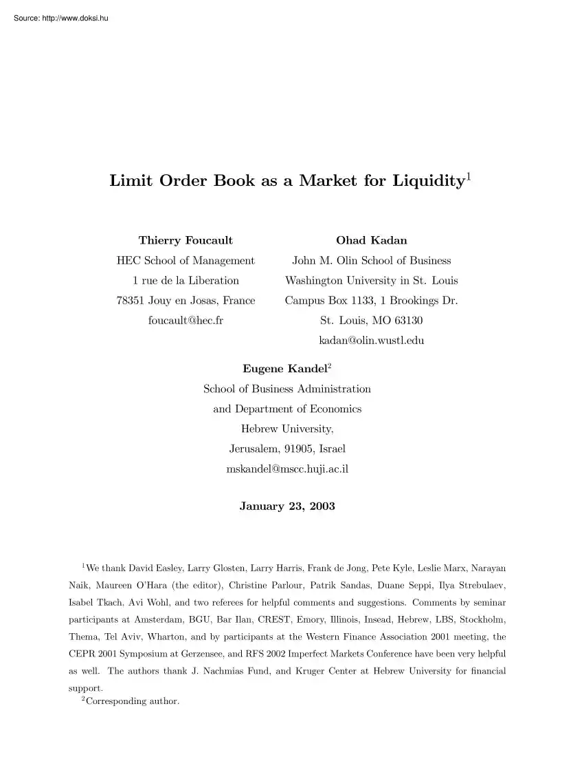
limit orders in Example 2, where r > 1. In fact, spread improvements are larger than one tick for all spreads on the equilibrium path in this case. In contrast, in Example 3, spread improvements are equal to one tick in most cases. Expected Waiting Time The expected waiting time function in Examples 2 and 3 is illustrated in Figure 1, which presents the expected waiting time of a limit order as a function of the spread it creates. In both examples the expected waiting time increases when we move from one reached spread to the next, while it remains constant over the spreads that are not reached in equilibrium. The expected waiting time is smaller at any spread in Example 3. This explains the differences in bidding strategies in Examples 2 and 3. When r < 1, patient traders are less aggressive because they expect a faster execution. Book Dynamics and Resiliency Figure 2 illustrates the evolution of the limit order book over 40 trader arrivals. We use the same realizations for
traders’ types in Examples 2 and 3 and look at the dynamics of the best quotes. Initially the spread is equal to K = 20 ticks This may be the situation of the book, for instance, after the arrival of several market orders. How fast does the spread revert to the competitive level? 15 16 The equilibrium strategies in Examples 2 and 3 follow from the formulae given in Proposition 5. To fully specify the equilibrium strategy, Table 2 presents the optimal actions for spreads on and off the equilibrium path. 18 Table 2 - Equilibrium Order Placement Strategies Current Example 1 Example 2 Example 3 Spread Type 1 Type 2 Type 1 Type 2 Type 1 Type 2 1 0 0 0 0 0 0 2 0 0 1 0 1 0 3 2 2 1 0 1 0 4 2 2 3 0 3 0 5 2 2 3 0 3 0 6 2 2 3 0 5 0 7 2 2 6 0 6 0 8 2 2 6 0 7 0 9 2 2 6 0 8 0 10 2 2 9 0 9 0 11 2 2 9 0 10 0 12 2 2 9 0 11 0 13 2 2 9 0 12 0 14 2 2 13 0 13 0 15 2 2 13 0 14 0 16
2 2 13 0 15 0 17 2 2 13 0 16 0 18 2 2 13 0 17 0 19 2 2 18 0 18 0 20 2 2 18 0 19 0 In both examples, the competitive spread (i.e, patient traders’ reservation spread) is 1 tick and can be posted in equilibrium (see Table 2). However, as is apparent from Figure 2, the competitive spread is reached much more quickly in Example 2 than in Example 3. In fact, in Example 3, the quoted spread remains much larger than the competitive spread during all 40 periods depicted in Figure 2. In contrast, in Example 2, the competitive spread is sometimes posted and the spread is frequently close to the competitive spread. Since the type realizations in both books are identical, this observation is due to the fact that, in Example 2, patient traders 19 Expected Waiting Time - T ( j ) 30 example 2 25 example 3 20 15 10 5 0 1 3 5 7 9 11 13 15 17 19 Submitted Spread ( j ) Figure 1: Expected Waiting Time use more aggressive limit orders in order to
speed up execution.17 This bidding behavior explains why the market appears much more resilient in Example 2 than in Example 3. Our measure indicates that the resiliency of the market is much larger in Example 2, R = 0.556 ' 002, than in Example 3, where R = 0.4517 ' 127 × 10−6 Summary: When traders are homogeneous, any deviation from the competitive spread is immediately corrected. This is not the case in general when traders are heterogeneous In the latter case, the market is more resilient when r ≥ 1 than when r < 1. Thus, although the equilibrium of the limit order market is unique, three patterns for the dynamics of the spread emerge: (a) strongly resilient, when traders are homogeneous, (b) resilient, when traders are heterogeneous and r ≥ 1 and (c) weakly resilient, when traders are heterogeneous and r < 1. 17 If type realizations were not held constant, an additional force would make small spreads more frequent when r ≥ 1. In this case, the
liquidity offered by the book is consumed less rapidly, since the likelihood of a market order is smaller than when r < 1. Thus the inside spread has more time to narrow between market order arrivals 20 Figure 2 - Book Simulation (same realizations of type arrivals for two examples) Example 2 - A Resilient Book ( r = 1.222) Period 1 2 3 4 5 6 7 8 9 10 11 12 13 14 15 16 17 18 19 20 21 22 23 24 25 26 27 28 29 30 31 32 33 34 35 36 37 38 39 40 Trader B2 S1 B1 S2 B2 S2 B1 S1 B2 S1 B2 S1 B1 S1 B2 S1 B1 S1 B1 S2 B1 S1 B1 S1 B2 S2 B1 S2 B1 S1 B1 S2 B2 S1 B2 S2 B2 S1 B1 S2 22 1/2 22 3/8 22 1/4 22 1/8 22 21 7/8 21 3/4 21 5/8 21 1/2 21 3/8 21 1/4 21 1/8 21 20 7/8 20 3/4 20 5/8 20 1/2 20 3/8 20 1/4 20 1/8 20 s s s s s s s s s s s s s s s s s s s s s s s s s s s s s s s s s s s s s s s s s s s s s s s s s s s s s s s s s s s s s s s s s s s s
s s s s s s s s s s s s s s s s s s s s b s b b b s b b s b b b s b b b b b b b b b b b b b s s s b b b b b b b b b b s b b b b b b b b b b b b b b b b b b b b b b b b b b b b b b b b b b b b b b b b b b b b b b b b b b b b b b b b b b b b b b b b b b b b b b b b b b b b b b b Example 3 - A Weakly Resilient Book ( r = 0.818 ) Period 1 2 3 4 5 6 7 8 9 10 11 12 13 14 15 16 17 18 19 20 21 22 23 24 25 26 27 28 29 30 31 32 33 34 35 36 37 38 39 40 Trader B2 S1 B1 S2 B2 S2 B1 S1 B2 S1 B2 S1 B1 S1 B2 S1 B1 S1 B1 S2 B1 S1 B1 S1 B2 S2 B1 S2 B1 S1 B1 S2 B2 S1 B2 S2 B2 S1 B1 S2 22 1/2 22 3/8 22 1/4 22 1/8 22 21 7/8 21 3/4 21 5/8 21 1/2 21 3/8 21 1/4 21 1/8 21 20 7/8 20 3/4 20 5/8 20 1/2 20 3/8 20 1/4 20 1/8 20 s s s s s s s s s s s s s s s s s s s s s s s s s s s s s
s s s s s s s s s s s s s s s s s s s s s s s s s s s s s s s s s s s s s s s s s s s s s s s s s s s s s s s s s s s s s s s s s s s s s s s s s s s s s s s s s s s s s s s s s s s s s s s s s s s s s s s s s s s s s s s s s s s s s b b b b b b b b b b b b b b b b b b b b b b b b b b b b b b b b b b b b b b b b b b b b b b b b b b b b b b b b b b b b b b b b b b b b b b b b b b b b b b b b b b b b b b b b b b b b b b b b b b b b b b b b b b b b b b b b b b b b b b b b b b b b b b b b b b b b b b b b b b b b b Legend: B1 - Patient buyer, B2 - Impatient buyer, S1 - Patient seller, S2 - Impatient seller b - a buyers limit order, s - a sellers limit order. b b b b b b b b b b b b b b b b b b b b 3.4 Distribution of Spreads In this section, we derive the probability distribution of the spread induced by equilibrium order placement strategies. We exclusively focus on the case in which traders are heterogeneous since this
is the only case in which transactions can take place at spreads different from the competitive spread. We show that the distribution of spreads depends on the composition of the trading population: small spreads are more frequent when r ≥ 1 than r < 1. This reflects the fact that markets dominated by patient traders (r ≥ 1) are more resilient than markets dominated by impatient traders (r < 1). From Proposition 3 we know that the spread can take q different values: n1 < n2 < . < nq in equilibrium. A patient trader submits an nh−1 -limit order when the spread is nh (h = 2, , q) and a market order when he faces a spread of n1 . An impatient trader always submits a market order (we maintain the assumption that sc = K). Thus, if the spread is nh (h = 2, , q − 1) the probability that the next observed spread will be nh−1 is θ, and the probability that it will be nh+1 is 1 − θ. If the spread is n1 all the traders submit market orders and the next observed
spread will be n2 with certainty. If the spread is K then it remains unchanged with probability 1 − θ (a market order), or decreases to nq−1 with probability θ (a limit order). Hence, the spread is a finite Markov chain with q ≥ 2 states. The q × q transition matrix of this Markov chain, denoted by W, is: W = 0 1 0 ··· 0 θ 0 1 − θ ··· 0 0 . . θ . . 0 . . ··· 0 . . 0 0 0 ··· 0 0 0 0 ··· θ 0 0 0 . . 1−θ 1−θ The j th entry in the hth row of this matrix gives the probability that the size of the spread becomes nj conditional on the spread having size nh (j, h = 1, ., q) The long-run probability distribution of the spread is given by the stationary probability distribution of this Markov chain.18 We denote the stationary probabilities by u1 , uq , where uh is the probability of a spread of size nh . 18 See
Feller (1968). 22 0.25 Probabilities 0.2 Example 2 Example 3 0.15 0.1 0.05 0 1 2 3 4 5 6 7 8 9 10 11 12 13 14 15 16 17 18 19 20 Spreads Figure 3: Equilibrium Spread Distribution Lemma 2 :The spread has a unique stationary probability distribution, which is given by: u1 = uh = θq−1 + θq−1 , q−i (1 − θ)i−2 i=2 θ Pq θq−h (1 − θ)h−2 Pq q−i (1 − θ)i−2 i=2 θ θq−1 + h = 2, ., q (10) (11) Figure 3 depicts the stationary distribution in Examples 2 and 3. Clearly, the distribution of spreads is skewed toward higher spreads in Example 3 (r < 1) and toward lower spreads in Example 2 (r > 1). This observation stems from the expressions for the stationary probabilities For h, h0 ∈ {2, 3, ., q} with h > h0 , Lemma 2 implies that uh uh 1 0 = rh −h , and = h−1 , uh0 u1 r (1 − θ) which yields the following corollary. Corollary 2 : For a given tick size and waiting costs: 1. If r < 1, uh > uh0 for 1 ≤ h0 < h ≤ q
Thus, the distribution of spreads is skewed towards higher spreads when r < 1. 23 2. If r > 1, uh < uh0 for 2 ≤ h0 < h ≤ q19 Thus, the distribution of spreads is skewed towards lower spreads when r > 1. The expected dollar spread is given by:20 ES m = q X uh nm h, (12) h=1 The smaller is the expected dollar spread, the more distant are transaction prices from the “boundaries” A and B. Thus, smaller bid-ask spreads are associated with higher profits to liquidity demanders (the impatient traders), since their market orders meet more advantageous prices. Using Equation (12), we find that the expected spread in Example 2 (r > 1) is smaller than in Example 3 (r < 1) ($1.05 vs $2) 4 Tick Size, Arrival Rate, and Waiting Cost In this section we explore the comparative statics with respect to three parameters: tick size, traders’ arrival rate, and traders’ waiting cost. In our model equilibrium spreads are determined by the ratio δλ1 (see
Propositions 1 and 5). For this reason the results on an increase in the arrival rate translate immediately to results on a decrease in the waiting costs δ1 . Thus we only analyze the effect of the order arrival rate to save space. For the same reason we restrict our attention to cases in which traders have different reservation spreads, i.e j1R < j2R We maintain our assumption that sc = K, so that impatient traders always choose market orders. 4.1 Tick Size and Resiliency The tick size (the minimum price variation) has been reduced in many markets in recent years. In this section we examine the effect of a change in the tick size in our model. We assume throughout that such a change does not affect the fundamentals of the security, hence it does not 19 The inequality, uh < uh0 , does not necessarily hold for h0 = 1, when r > 1. Actually the smallest inside spread can only be reached from higher spreads, while other spreads can be reached from both directions (nq =
K can be reached either from nq−1 or from nq itself). This implies that the probability of observing the smallest possible spread is relatively small for all values of r. 20 Recall that a superscript “m” indicates variables expressed in monetary terms, rather than in number of ticks (i.e nm h = nh ∆). 24 change the monetary boundaries Am = A∆ and B m = B∆. This means that K m = K∆ is fixed independently of the value of the tick size. It has often been argued that a decrease in the tick size would reduce the average dollar spread. We show below that this claim does not necessarily hold true in our model, because a reduction in the tick size tends to impair market resiliency.21 We demonstrate that imposing a positive tick size in a weakly resilient market tends to enhance resiliency and consequently lower the expected spread. To better convey the intuition, it is useful to consider the polar case in which there is no minimum price variation (i.e, ∆ = 0) In this case
prices and spreads must be expressed in monetary terms. Thus in what follows, we index all spreads by a superscript “m” to indicate that they are expressed in dollar terms. When the tick size is zero, a trader’s reservation spread is exactly equal to his per period waiting cost, i.e jiRm = δλi (i ∈ {1, 2}) We denote by K m the largest possible monetary spread. Finally T (j m ) denotes the expected waiting time for a limit def m λ−δ1 c order trader who creates a spread of j m dollars. Let rc = K K m λ+δ1 . Notice that 0 < r ≤ 1 since j1Rm < K m by assumption (Equation (3)). The next proposition extends Propositions 4 and 5 to the case in which there is no mandatory minimum price variation. Proposition 6 : Suppose that ∆ = 0. If r > rc and δ1 > 0, the equilibrium is as follows:22 1. The impatient traders never submit a limit order δ1 m m m m m 2. There exist q0 spreads nm 1 < n2 < . < nq0 , with n1 = λ and nq0 = K such that a patient m m
trader submits an nm h -limit order when he faces a spread in (nh , nh+1 ] and a market order when he faces a spread smaller than or equal to nm 1 . (The expression for q0 is given in Appendix A). m m m h−1 ) δ1 , for h = 2, .q − 1 and 3. The spreads are: nm 0 h = nh−1 + Ψh (0), where Ψh (0) = (2r λ the stationary probability of the hth spread is uh , as given in Section 3.4 21 See Seppi (1997), Harris (1998), Goldstein and Kavajecz (2000), Christie, Harris, and Kandel (2002), and Kadan (2002) for arguments for and against the reduction in the tick size in various market structures. The idea that a reduction in the tick size can impair market resiliency is new to our paper. 22 If r < rc then spread improvements are so small that the competitive spread is never achieved, and resiliency is zero. We discuss this case later The same problem arises if patient traders’ waiting cost is zero 25 h Ph−1 k i 1 1 m for 4. The expected waiting time function is such that
(1) T (nm 1 ) = λ , (2) T (nh ) = λ 1 + 2 k=1 r m m m h = 2, ., q0 − 1 and (3) T (j m ) = T (nm h ) for j ∈ (nh−1 , nh ]. Proposition 6 shows that when r > rc the equilibria with or without a minimum price variation are qualitatively similar. The smallest possible spread is patient traders’ per period waiting cost, i.e δλ1 In contrast, when ∆ > 0, it is equal to this cost rounded up to the nearest tick Thus the competitive spread is larger when a minimum price variation is enforced. This rounding effect th propagates to all equilibrium spreads. To make this statement formal, let nm h (∆) denote the h smallest spread in the set of spreads on the equilibrium path when the tick size is ∆ ≥ 0, and let q∆ be the number of equilibrium spreads in this set. The following holds Corollary 3 “Rounding effect”: Suppose r > rc . Then in equilibrium: (1) q∆ ≤ q0 , (2) nm h (0) ≤ m m nm h (∆), for h < q∆ , and (3) nh (0) ≤ nq∆ (∆) for q∆
≤ h ≤ q0 . This means that the support of possible spreads when the tick size is zero is shifted to the left compared to the support of possible spreads when the tick size is strictly positive. Given this result, it is tempting to conclude that the average spread is always minimized when there is no minimum price variation. This indeed has been the conventional wisdom behind the tick size reductions in many markets. We show below that this reasoning does not draw the whole picture because it ignores the impact of the tick size on the dynamics of the spread in between transactions. When r > rc and δ1 > 0, in zero-tick equilibrium, traders improve the spread by more than 23 Intuitively, patient traders improve the quote by a an infinitesimal amount (Ψm h (0) > 0). non-infinitesimal amount to speed up execution. However, as r decreases, spread improvements become smaller and smaller: traders bid less aggressively since market orders arrive more frequently (see the
discussion following Proposition 5). When ∆ > 0 price improvements can never be smaller than the tick size; thus for small values of r traders improve prices by more than they would in absence of a minimum price variation. We refer to this effect as being the “spread improvement effect”. The spread improvement effect works to increase the speed at which spread narrows in between transactions. For this reason imposing a minimum price variation helps to 23 Traders must improve upon prevailing quotes (Assumption A.2) However when the tick size is zero, they can improve by an arbitrarily small amount. Proposition 6 shows that they do not take advantage of this possibility when r > rc . 26 make the market more resilient. This intuition can be made more rigorous by using the measure of market resiliency, R, defined in Section 3.22 Corollary 4 (tick size and resiliency): Other things being equal, the resiliency of the limit order market (R) is always larger when there
is a minimum price variation than in the absence of a minimum price variation. Furthermore, the resiliency of the market (R) approaches zero as r approaches rc in the absence of a minimum price variation, whereas it is always strictly greater than zero when a minimum price variation is imposed. Intuitively, as r approaches rc from above, the spread improvements become infinitesimal when the spread is large (e.g equal to K) Thus the quotes are always set arbitrarily close to the largest possible ask price, A, or the smallest possible bid price, B. This explains why, in the absence of a minimum price variation, the resiliency of the market vanishes when r goes to rc . Imposing a minimum price variation in this kind of weakly resilient markets is a way to avoid this pathological situation, because it forces traders to improve by non-infinitesimal amounts. Thus, intuitively, imposing a minimum price variation can be a way to reduce the expected spread, despite the rounding effect,
because it makes the market more resilient. We demonstrate this claim by providing a numerical example. The values of the parameters are as in Example 3 except that r = 0.97 (ie θ = 049, and the market is weakly resilient), so that the condition r > rc is satisfied.24 Table 3 gives all the monetary spreads on the equilibrium path for two different values of the tick size: (1) ∆ = 0 and (2) ∆ = 0.0625 The two last lines of the table give the expected spread and the resiliency obtained for each regime. First, observe the “rounding effect” - the thirteen smallest spreads are lower when ∆ = 0, than in the case of ∆ = 0.0625 Second, observe the “spread improvement effect” - the spread reduction is quicker for every spread level if a minimum price variation is enforced. This explains why market resiliency is smaller when there is no minimum price variation. For this reason, the expected spread turns out to be larger in this case ($1.58 instead of $148) 24 Given the
values of the parameters rc ≈ 0.92 27 Table 3 - Rounding and Spread Improvement Effects (Parameter Values: λ = 1, K m = 2.5, δ1 = 01, δ2 = 025, r = 097) h nm h (∆ = 0) nm h (∆ = 0.0625) 1 $0.1 $0.125 2 $0.294 $0.375 3 $0.482 $0.625 4 $0.665 $0.813 5 $0.842 $1 6 $1.014 $1.188 7 $1.181 $1.375 8 $1.343 $1.563 9 $1.5 $1.75 10 $1.652 $1.938 11 $1.799 $2.125 12 $1.942 $2.313 13 $2.081 $2.5 14 $2.216 NA 15 $2.347 NA 16 $2.474 NA 17 $2.5 NA Expected Spread $1.58 $1.48 Resiliency 1.1 × 10⁻⁵ 1.9 × 10⁻⁴ So far we have compared a situation with and without a mandatory minimum price variation. More generally, the “spread improvement” effect implies that the expected spread does not necessarily decrease when the tick size is reduced. In order to see this point, consider Table 4 It 1 1 1 demonstrates which of the following tick sizes, { 100 , 16 , 8 }, minimizes the expected spread for dif1 ferent values of r.
Consistent with the above argument ∆ = 100 does not minimize the expected spread for low values of r. However as r increases, inducing traders to make large improvements by imposing a large minimum price variation becomes less effective, since they already submit aggressive orders. For this reason, the “spread improvement effect” becomes of second order compared to the “rounding effect”. In fact Table 4 shows that the tick size which minimizes 28 the expected spread decreases with r and that once r ≥ 1 the expected spread is minimized at 1 ∆ = 100 . Table 4 - The Tick Size Minimizing the Expected Spread 1 1 1 (Parameter Values: λ = 1, K m = 2.5, δ1 = 01, δ2 = 025, ∆ ∈ { 100 , 16 , 8 }) r 0.7 0.8 0.9 0.93 0.97 1 1.1 1.2 1.3 ∆∗ 1 8 1 8 1 8 1 16 1 16 1 100 1 100 1 100 1 100 Finally we briefly discuss the case in which r < rc . In this case, traders improve upon large spreads by an infinitesimal amount. Thus the quotes are always
set arbitrarily close to the largest possible ask price, A, or the smallest possible bid price, B.25 Thus market resiliency is zero, as when r goes to rc . Imposing a minimum price variation is a way to restore market resiliency since spread improvements are non-infinitesimal as soon as ∆ > 0 (Proposition 5). To sum up, reducing or even eliminating the tick size may or may not reduce the average spread. The impact depends on the proportion of patient traders in the market, r Many empirical papers have found a decline in the average quoted spreads following a reduction in tick size. These papers, however, do not control for the ratio of patient to impatient traders One difficulty of course is that this ratio cannot be directly observed. In Section 5, we argue that the proportion of patient traders is likely to decrease over the trading day. In this case, the impact of a decrease in the tick size on the quoted spread should vary throughout the trading day. Specifically, a decrease
in the tick size may increase the average spread at the end of the trading day. To the best of our knowledge, there exists no test of this hypothesis 4.2 Fast vs. Slow Markets In this section, we analyze the effect of orders’ arrival rate (λ) on the dynamics of the spread and the expected spread. We compare two markets, F and S, which differ only with respect to orders’ arrival rate, λ. Specifically, λF > λS , which implies that the average waiting time between orders in market F is smaller than in market S. Thus, other things being equal, events (orders and trades) happen faster in clock time in market F . For this reason, we refer to market 25 This would also be the case if patient traders’ waiting cost were equal to zero (δ1 = 0). When r < rc or δ1 = 0, the equilibrium (when there is no minimum price variation) is difficult to describe formally since traders improve upon prevailing quotes by an infinitesimal, but strictly positive, amount. 29 F as a
fast market and market S as a slow market. Proposition 5 and Corollary 1 immediately yield the next result. Corollary 5 : Consider two markets with differing orders’ arrival rates: λF > λS . Then: 1. The spreads on the equilibrium path in markets F and S are such that: (1) nh (λF ) ≤ nh (λS ), for h < qS and (2) nh (λF ) ≤ K, for qS ≤ h ≤ qF . This means that the support of possible spreads in the fast market is shifted to the left compared to the support of possible spreads in the slow market. 2. The slow market is more resilient than the fast market The economic intuition of these results is as follows. On the one hand, the waiting time of a trader with a given priority level in the queue of limit orders is smaller in the fast market (see Proposition 4), thus patient traders require a smaller compensation for waiting. This effect explains the first part of the proposition. On the other hand, spread improvements are larger and the spread narrows more quickly
in the slow market (see the discussion following Proposition 5). Hence the slow market is more resilient. These two effects have an opposite impact on the average spread. Unfortunately it is not possible to determine analytically which effect is dominant. Simulations show that a decrease in the order arrival rate enlarges the expected spread for a wide range of parameters’ values (i.e the first effect dominates) but not always. Table 5 illustrates this claim by reporting the equilibrium expected dollar spread for various pairs (θ, λ).26 If we assume that all the assumed values for the pairs (θ, λ) have the same probability, the correlation between the average spread and the order arrival rate is negative and equal to −0.24 This indicates that overall the average spread tends to decline when the order arrival rate increases. Notice that the effects associated with a change in λ are very similar to those associated with a change in the tick size. Two forces contribute to a
small average spread: (i) small frictional costs on the one hand (a small tick, small waiting time between arrivals) and (ii) large spread improvements. Our analysis points out that factors which lessen frictional costs may reduce spread improvements, resulting in less resilient markets and eventually higher spreads. 26 The condition sc = K holds for all parameter values considered in this table. Hence, we use Proposition 5, Lemma 2 and Equation (12) to compute the equilibrium spreads. 30 Table 5 - Expected Spreads and Order Arrival Rates (Parameter Values: ∆ = 0.125, K m = 25, δ1 = 01, δ2 = 025) θ 0.35 0.4 0.45 0.5 0.55 0.6 0.65 1 2.35 2.25 2 1.42 1.05 0.91 0.79 4/5 2.3542 2.251 2.02 1.46 1.20 1.18 1.01 2/3 2.3542 2.252 2.02 1.46 1.17 1.11 1.145 1/2 2.3542 2.2532 2.03 1.56 1.34 1.24 1.146 1/3 2.3543 2.2584 1.94 1.51 1.56 1.44 1.41 1/5 2.3539 2.1 1.98 1.82 1.80 1.89 1.76 λ 5 Empirical Implications Trading Intensity
and Spreads. In his pioneering paper, Demsetz (1968) argues that in the presence of waiting costs, the spread and the transaction rate should be inversely related. He writes (p 41): “The fundamental force working to reduce the spread is the time rate of transactions. The greater the frequency of transacting, the lower will be the cost of waiting in a queue of specified length and, therefore, the lower will be the spreads that traders are willing to submit to preempt positions in the trading queue.” In our framework both the transaction rate and the spreads are endogenous. In what follows, we study the relation between the spread and the transaction rate to test Demsetz’s conjecture. Our main finding is that the relationship between the spread and the transaction rate is not necessarily negative. This depends on whether or not, we control for the effect of the order arrival rate. Denote by D̄ the unconditional duration, i.e the expected time elapsing between two consecutive
transactions Clearly, transaction frequency is inversely related to D̄ Similarly let D̄h denote the expected time elapsing between two consecutive transactions, conditional on the first transaction taking place when the spread is nh . We refer to this variable as a conditional duration Analyzing the effect of the exogenous parameters on the conditional durations helps to understand the effect of these parameters on the unconditional duration. We proceed to derive 31 the two duration measures. Corollary 6 : In equilibrium, the conditional duration is: D̄h = 1 − θh+1 1 − θq for 1 ≤ h < q; and D̄q = , λ(1 − θ) λ(1 − θ) (13) while the unconditional duration is: D̄ = · ¸ 1 θq 1 − Pq . q−h (1 − θ)h−1 λ(1 − θ) h=1 θ (14) Interestingly, Equations (13) and (14) reveal that the order arrival rate, λ, is not the only determinant of conditional durations between transactions. The proportion of patient traders, θ, plays an important role as
well. As expected, each conditional duration declines in the arrival rate, λ, and increases in the proportion of patient traders, θ. Intuitively, the larger is θ, the larger is the probability of arrival of many consecutive patient traders, which postpone the next transaction. The unconditional duration depends not only on the conditional durations but also on the probability distribution of spreads. This makes it very difficult to study analytically the effects of the order arrival rate and the proportion of patient traders on the unconditional duration. To gain intuition, Table 6 calculates the unconditional duration for different values of θ and λ, holding other parameters constant. Table 6 - Unconditional Duration Between Trades (clock time) (Parameters Values: ∆ = 0.125, K m = 25, δ1 = 01, δ2 = 025) θ 0.35 0.4 0.45 0.5 0.55 0.6 0.65 1 1.53 1.66 1.81 1.90 1.92 1.93 1.93 4/5 1.92 2.08 2.26 2.32 2.38 2.41 2.41 2/3 2.3 2.49 2.71 2.78 2.81 2.83
2.9 1/2 3.07 3.33 3.60 3.67 3.75 3.78 3.87 1/3 4.61 4.99 5.27 5.29 5.5 5.5 5.65 1/5 7.68 8.10 8.42 8.54 8.87 9.17 8.98 λ As the conditional durations, the unconditional duration declines in the order arrival rate, λ. In almost all cases, the unconditional duration increases with the proportion of patient traders, 32 θ. This property does not always hold, however because an increase in θ has two opposite effects on the unconditional duration. On the one hand, a higher proportion of patient traders increases each conditional duration and thus works to enlarge the unconditional duration. But a higher proportion of patient traders also increases market resiliency (see Section 3). This effect increases the frequency of lower spreads. Now, Equation (13) implies that the duration between trades is smaller conditional on the spread being small (Dh increases with h). Thus the overall effect of θ on the unconditional duration is ambiguous. Inspection of
Table 6 shows that the first effect dominates in many cases (i.e, the unconditional duration increases with θ) but not always These findings have several implications for empirical research. First, two markets with identical order arrival rates may still exhibit very different levels of activity, if the proportion of patient traders in these markets differs. Moreover, an increase in the order arrival rate does not necessarily lead to a proportional increase in transaction frequency, as often assumed in time deformation models (see Hasbrouck (1999) for a discussion of these models). Suppose, for instance, that a common factor raises the order arrival rate and the proportion of patient traders. Then the increase in the order arrival rate will not necessarily be associated with an increase in the transaction frequency. In any case, the frequencies of orders and trades will be less than perfectly correlated. Hasbrouck (1999) shows that indeed these frequencies are not highly
correlated, in particular over short horizons. Second, for a given order arrival rate, variations in the proportion of patient traders create a positive relationship between transaction frequencies and spreads. Recall that a decrease in the proportion of patient traders has two effects. First, it reduces limit order traders’ aggressiveness Second, it yields a larger transactions rate since impatient traders submit market orders The combination of these two effects generates a positive correlation between spreads and the transaction rate. The simulations in Tables 5 and 6 illustrate this point In fact, if we assume that all the assumed values of θ have the same probability, the correlation between the average spread and the transaction frequency (defined as the inverse of the unconditional duration) varies between 0.7 when λ = 1/5, and 094 when λ = 4/5 Finally, for a given proportion of patient traders, variations in the order arrival rate tend to create a negative relationship
between the expected spread and the transaction frequency. Actually, as explained in Section 4.2, an increase in λ often results in smaller average spreads On the other hand, it raises the transaction frequency. The combination of these effects results 33 in a negative correlation between the transaction rate and the average spread. This is not always the case, however, since the relationship between the order arrival rate and the average spread is non-monotonic (see Section 4.2) For instance, if we assume that the chosen values of λ in Tables 5 and 6 are equally probable, then the correlation between the expected spread and the transaction rate is negative for all values of θ, except θ = 0.4 and θ = 045 Demsetz (1968) and several subsequent studies (e.g Harris 1994) have found a negative crosssectional relation between the number of transactions per day (a measure of the transaction rate) and the average spread. This empirical finding is not inconsistent with our results
because these studies have not controlled for the effect of the order arrival rate. In fact, for the examples considered in Table 5 and 6, the correlation between the average spread and the transaction frequency is negative. The exact prediction of our model is that the spread should be positively related to the transaction rate, controlling for the order arrival rate. Testing this prediction offers a way to obtain a better economic understanding of the empirical correlations between spreads and transaction rates. Intraday Patterns. It is well known that spreads and trading activity follow a reversed J-shaped pattern in many limit order markets.27 This pattern has proved difficult to explain in asymmetric information models. For instance, in Admati and Pfleiderer (1988), traders concentrate their transactions at times where spreads are small, not large. Furthermore, Madhavan, Richardson and Roomans (1997) empirically show that the adverse selection component of the spread declines
throughout the day. Finally, Chung et al (1999) find that intraday patterns on the NYSE are mainly due to intraday variations in spread set by limit order traders rather than by the specialist. This finding does not support inventory-based explanations for the rise of the spread towards the end of the trading day. We suggest that the intraday patterns are driven by the systematic variations in the proportion of patient traders during the day. In general, inability to trade overnight is a binding constraint for many investors. Moreover, many institutions mark to market at the end of the day; thus they prefer to trade closer to that deadline. This also creates pressure towards the end of the 27 For recent evidence see Biais, Hillion and Spatt (1995) for the Paris Bourse or Chung, Van Ness and Van Ness (1999) for the NYSE. 34 day.28 If this is the case, the proportion of impatient traders and, thereby, limit order fill rate should steadily increase towards the end of the day. The
model predicts that spreads and the transaction frequency should be higher towards the end of the day (see the discussion above), which is consistent with the stylized facts. Furthermore, the aggressiveness of limit order traders should decline towards the close, resulting in less resilient markets (see the discussion following Proposition 5). To the best of our knowledge, this prediction (markets are less resilient in the last part of the trading day) has not been tested yet. Pagano and Schwartz (2002) show that an introduction of a closing auction in Paris Bourse caused a reduction in spreads in the last half hour of trading. Traditional theory would predict the opposite as the closing auction is likely to draw liquidity away from the continuous market. We, however, interpret this event as an introduction of a new trading opportunity, which increases the patience of traders earlier; thus causing the spread reduction. Spread Improvements. Several empirical studies of limit order
markets have analyzed the impact of the state of the book on the order flow (e.g Biais et al (1995), Griffith et al(2000) or Benston, Irvine and Kandel (2001)). These studies classify new orders by their aggressiveness, defined by the position of the price of a limit order relative to prevailing quotes. For instance, a limit order within the prevailing quotes is more aggressive than a limit order behind the best quotes. Our paper suggests a measure of aggressiveness of the limit orders: the amount by which limit order traders improve upon prevailing quotes. Proposition 5 has the following implication Corollary 7 : The amount by which limit order traders improve upon the prevailing quotes depends on the size of the inside spread. This amount increases with the size of the spread when r > 1, and decreases with the size of the spread when r < 1. Recall that the price concession a trader is willing to offer is equal to the reduction in the waiting time he obtains (Equation (8)).
When r > 1, the waiting time function is “convex” in the sense that (T (nh ) − T (nh−1 )) increases with h. Hence, liquidity suppliers are willing to offer larger spread improvements when the spread is large. When r < 1, the waiting time function is “concave” (i.e (T (nh ) − T (nh−1 )) decreases in h); thus liquidity suppliers offer larger spread 28 Recent experimental findings by Bloomfield, O’Hara, and Saar (2002) support this intuition. They show that liquidity traders who are assigned a trading target switch form limit to market orders at the end of trading sessions. 35 improvements at small spreads. If the proportion of patient traders decreases over the trading day then the direction of the relationship between spread improvements and the size of the spread may change over time during the trading day. Engle and Patton (2001) find that the size of the spread is an important determinant of the dynamics of bid and ask prices for stocks listed on the
NYSE. Their time-series analysis shows that the change in the log of the best ask (bid) price is negatively (positively) related to the size of the spread. This means that the amount by which traders improve upon prevailing quotes is related to the size of the spread, as predicted by the model. The model yields predictions for the cross-sectional variation of spread improvements as well. For example, Proposition 5 implies a negative relation between spread improvements and the order arrival rate, which may vary across stocks. Also, Proposition 5 shows that quote improvements decline in θ. We expect stocks that belong to a widely followed index to attract more impatient traders than other stocks, since many index fund managers must trade rapidly to minimize their tracking error. Hence, controlling for other stock characteristics, eg, λ, we expect spread improvements to be smaller for stocks, which belong to an index. Time-to-execution. Lo, McKinlay and Zhang (2001) emphasize the need
of statistical models of limit order execution times to assist traders in their choice between market and limit orders. An equilibrium model, such as this one, provides helpful insights for specifications of these models. In particular, we find that the time-to-execution for limit orders decreases with the order arrival rate, and increases with the proportion of patient traders (see Equation (5) and Figure 1). For a given order arrival rate, the transaction frequency is negatively related to the proportion of patient traders, and thus can serve as a proxy for θ. This suggests that econometric models of time-to-execution should include the order arrival rate and the transaction frequency as explanatory variables. These variables should be negatively related to time-to-execution Lo, McKinlay and Zhang (2001) find that time-to-execution decreases with various measures of trading intensity. They do not consider the effect of the order arrival rate, however They also point out that there
is a large variation in mean time-to-execution across stocks. According to our model, these variations could be explained by the fact that stocks differ with respect to the order arrival rate, maybe because they differ with respect to the number of shareholders. 36 6 Robustness Recall our assumptions regarding the trading process: A.1 - no order cancellations and resubmissions; A2 - limit orders cannot queue at or behind the best quotes, and A3 - buyers and sellers alternate. Since these assumptions are clearly unrealistic, the robustness of the implications obtained in our model is a concern We address this concern in this section, by first stating the technical reasons for these assumptions, and then arguing that our results are not an artifact of these assumptions. We present conditions under which our non-queueing restriction becomes non-binding. We also show, using examples, that the main properties of the model (described in Section 3) persist when we relax the
assumption that buyers and sellers alternate. Overall these robustness tests show that our main results are not driven by the technical assumptions, and that the economic intuitions are not changed when these assumptions are relaxed. 6.1 Cancellations and Resubmissions To the best of our knowledge there are no theoretical papers that allow for strategic cancellations and resubmissions of orders in a dynamic game; such a game is just too complex to analyze.29 We have not found the solution to this problem, thus we must also assume that our traders make one strategic decision only. Hollifield, Miller, Sandås and Slive (2002) take into account the possibility that traders cancel their orders. Their modeling approach consists in assuming that cancellations occur at random points in time after the initial submission. Unfortunately it is not possible to proceed in this way here since all traders must eventually carry out their desired transaction in our framework. Thus we would need to
arbitrarily specify the payoff of a trader in case of cancellation. Consequently, we do not engage in this exercise. Hence one limitation of our model is that it cannot explain why traders cancel or modify their orders. In reality most cancellations seem to stem from a particular behavior that we do not seek to study in this paper. Hasbrouck and Saar (2002) show that the majority of the limit orders submitted on Island ECN are cancelled, and the majority of those are cancelled within two 29 Harris (1998) studies the optimal dynamic order submission strategies in a partial equilibrium set-up (that is with an exogenous order flow). Even in this case, allowing traders to cancell and resubmit their orders is quite complex. 37 seconds after submission. These, so called “fleeting” orders seek liquidity rather than provide it, and their execution rates are very low. Many other cancelled limit orders were placed deep behind the best quote in hopes of a lucky execution. Neither one
of these order types should affect our conclusions. Tkach (2002) studies the limit order submission of the 100 most liquid stocks traded on the Tel Aviv Stock Exchange. The prevailing regulatory and institutional features do not induce “fleeting” orders; nevertheless, she shows that almost 40% of limit orders are cancelled. Out of these less than 30% are price improving limit orders that we study. Moreover, the median time to cancellation is 11 minutes, and over 11% of all cancelled orders cancel within a minute of submission. This is a short time, given the low volume in most of these stocks They represent a different phenomenon, which is outside the focus of this model. 6.2 Queuing at the Inside Quotes We have assumed that traders cannot place limit orders at or behind the existing inside quotes. In reality, such quotes are allowed and used. Allowing traders to queue at the best quotes cannot accelerate the rate at which the spread narrows between transactions, but it may
reduce it. Thus, allowing traders to queue results in less competitive and less resilient limit order markets, other things being equal. This, however, should not invalidate the findings that (i) an increase in the proportion of patient traders or (ii) a decrease in the order arrival rate yield more resilient and more competitive limit order markets. Actually, traders’ willingness to queue must be smaller when time-to-executions are large. Now, time-to-executions enlarges when the proportion of patient traders becomes larger or when the order arrival rate becomes smaller. For these reasons, the number of limit orders placed at a given price will decrease in these two cases. This means that spreads will narrow more quickly when the proportion of patient traders increases or the order arrival rate decreases, even when queuing is an option. If the previous intuition is correct, traders should decide not to queue at all when the proportion of patient traders is large enough or the order
arrival rate is small enough. In this case, the equilibrium is exactly as described in Section 3. The next proposition shows that this intuition is correct assuming that time priority is enforced, i.e limit orders entered first at a given price are executed first. Proposition 7 : Suppose traders are heterogeneous and are allowed to queue at the inside quotes 38 subject to a strict time priority. Then if λ∆ ≤ 2 [1 + θ(2 − θ)] , δ1 (15) the equilibrium when traders are not allowed to queue (see Section 3) is an equilibrium in this setting as well. Suppose that traders use the trading strategies described in Section 3, and give them the freedom to queue at the best quotes. Under Condition (15), traders prefer to submit limit orders improving upon the inside quotes rather than queuing. Hence, traders’ strategies form an equilibrium even though traders have the possibility to queue. Observe that the R.HS of Condition (15) increases with θ (taking values between 2 and
4) This means that traders will not queue (and markets will be more resilient) when the proportion of patient traders is large enough, as conjectured. Furthermore, the LHS increases with the order arrival rate, λ. This means that traders will not queue when the order arrival rate is small enough, as conjectured as well. Finally, queuing is never optimal when the tick size (∆) is sufficiently small, since liquidity providers can jump ahead of the queue at a low cost. This reasoning suggests that the number of limit orders placed at the same price should have decreased following tick size reductions. Finally, it is worth stressing that Condition (15) is satisfied in all the numerical examples we gave in the paper. It follows that the possibility of queuing does not per se invalidate our comparative statics, in particular those regarding the effect of the tick size. 6.3 Buyers and Sellers Arrive Randomly When buyers and sellers alternate, the expected waiting time function has a
recursive structure. This property considerably simplifies the analysis of the trading game because we can solve for the equilibrium order placement strategies by backward induction (see the discussion following Lemma 1). In Appendix B we present a simple setting that allows us to study our game, assuming that every arriving trader can be either a buyer or a seller with equal probability. In this appendix we explain why it is no longer possible to obtain a recursive expression for the expected waiting time. Furthermore we show that the waiting time for a given limit order depends on the entire state of the book when the order is placed and not only on the spread created by the limit 39 order. While these technical issues preclude any general analytical solution to the problem, we demonstrate below using examples that the basic economic intuitions of our model persist. As the waiting time function is not recursive, we cannot solve for the equilibrium strategies using backward
induction. Rather we have to employ the following solution method First, we “guess” (conjecture) equilibrium order placement strategies for patient and impatient traders. Second we use the conjectured equilibrium strategies in order to calculate expected waiting times of each possible limit order in each possible state of the book. This task is tedious and requires solving K(K + 1)/2 simultaneous linear equations, where K = A − B is the number of possible ticks in the book.30 Third, we check that the “guessed” strategies are indeed optimal given the expected waiting times computed in the second step. If it turns out that these strategies are not optimal one has to repeat all these steps until an equilibrium is found. For small levels of K the procedure described above is feasible, though highly tedious. We choose the case of K = 4 to demonstrate the robustness of our results. This choice of K allows for different levels of spread improvements. For example, when the spread
has 3 ticks, a trader can improve upon prevailing quotes by either 1 tick (small improvement) or 2 ticks (large improvement) or submit a market order. This allows us to show that limit order traders’ aggressiveness depends on θ, as in the baseline model. In order to illustrate this point, we present below the results of three examples corresponding to the three resiliency levels defined in the paper. The detailed presentation and solution of these examples is relegated to Appendix B. We show that the equilibrium has the same properties as the equilibrium obtained when buyers and sellers alternate. In particular, limit order traders place more aggressive orders and thereby the market is more resilient when the proportion of patient traders is large. Example 4 - A Strongly Resilient Book (homogenous traders). Set K = 4, ∆ = 0.125, δ1 = δ2 = 005, and assume that each arrival is either a buyer or a seller with equal probabilities. Traders are homogenous, hence θ has no role in this
example The following order placement strategy constitutes an equilibrium (see Appendix B): (i) when the spread is larger than 1 tick, buyers and sellers of both types submit a 1-limit order and (ii) when the spread is equal to 1 tick, both submit a market order. This equilibrium is identical to the homogeneous equilibrium in Proposition 1. Indeed, after a transaction, the spread increases (to 4 ticks) but it 30 The number of equations is large because the waiting function depends on the entire state of the book. 40 reverts to traders’ reservation spread (1 tick) before the next transaction. This market is therefore strongly resilient (R = 1). Example 5 - A Resilient Book (heterogenous traders, large θ). Set: ∆ = 0125, K = 4, θ = 0.7, λ = 1, δ1 = 002, and δ2 = 01, and assume that each arrival is either a buyer or a seller with equal probabilities. The following order placement strategies constitute an equilibrium (see Appendix B). An impatient trader always submits a
market order A patient trader submits (i) a 2-limit order when the spread is equal to 3 or 4 ticks, (ii) a 1-limit order when the spread is equal to 2 ticks and (iii) a market order when the spread is equal to 1 tick. The resiliency of the market is R = 0.49 Example 6 - A Weakly Resilient Book (heterogenous traders, small θ). Set: ∆ = 0.125, K = 4, θ = 03, λ = 1, δ1 = 002, and δ2 = 01, and assume that each arrival is either a buyer or a seller with equal probabilities. The following order placement strategies constitute an equilibrium (see Appendix B). An impatient trader always submits a market order When the spread is larger than 1 tick, a patient trader places a limit order improving the spread by 1 tick. When the spread is equal to 1 tick, a patient trader places a market order. The resiliency of the market is R = 0.027 Consider the case in which the spread is equal to 4 ticks and a patient trader arrives in the market. In Example 5, the trader improves upon prevailing
quotes by 2 ticks whereas in Example 6 he improves by only one tick. Thus, as in the baseline model, limit order traders use a more aggressive bidding strategy when the proportion of patient traders is large (Example 5). The economic intuition is exactly the same as when buyers and sellers alternate. Limit order traders bid more aggressively when θ is large because their waiting times are larger, other things equal (the waiting times of each limit order are derived in Appendix B). It follows that the resiliency of the market is larger when the proportion of patient traders is large (Example 5). Furthermore we show in Appendix B that the stationary distribution of spreads is skewed towards small (resp. large) spreads in Example 5 (resp. Example 6) Consequently the average spread is smaller in the market dominated by patient traders: the average spread is equal to $0.22 in Example 5 and $0.375 in Example 6 These examples demonstrate that relaxing the alternating arrival assumption does
not change the conclusions obtained when buyers and sellers alternate. The driving force of our model is that limit order traders react to exogenous increases in their waiting costs by submitting more 41 aggressive orders. This basic economic intuition does not hinge on the assumption that buyers and sellers alternate. However, relaxing this assumption prevents us from solving the model in general. We view our model as an elegant way to by-pass this problem without losing much of the economic intuitions. 7 Conclusions We consider a model of price formation in a limit order market. Traders in our model need to trade for exogenous reasons and differ in terms of impatience. Upon arrival they decide to submit a market order or a limit order. This decision is driven by a trade-off between the cost of immediacy and the cost of delayed execution, as first suggested by Demsetz (1968). Under simplifying assumptions we derive the equilibrium order placement strategies. We find that
traders submit more aggressive limit orders when the proportion of patient traders increases or the arrival rate decreases. For this reason, markets with a relatively high proportion of patient traders or a relatively small order arrival rate are more resilient. We also show that a reduction in the tick size impairs market resiliency, thus under some circumstances it may increase the average spread. The model generates many testable predictions, such as: (i) a positive relationship between trading frequency and the spread sizes, controlling for the order arrival rate; (ii) markets with a high order arrival rate are less resilient, but feature smaller spreads; (iii) limit order aggressiveness can be positively or negatively related to the size of the spread depending on whether patient or impatient traders dominate the trading population; (iv) spreads and trading frequency should increase over the course of the trading day, while limit order aggressiveness should decline towards the end
of the day. Our model suggests that a limit order market will be quite illiquid (featuring a large average spread and lacking resiliency) when the proportion of impatient traders is large. In this case, designated liquidity suppliers may drastically improve the quality of the market. The effect of designated liquidity suppliers on the equilibrium described in this paper is a possible direction for future research. 42 References [1] Admati A., and P Pfleiderer (1988), A Theory of Intraday Patterns : Volume and Price Variability, Review of Financial Studies, 1, Spring, 3-40. [2] Angel, J., (1994), Limit versus Market Order, working paper, Georgetown University [3] Benston, G, P. Irvine, and E Kandel (2001), Liquidity Beyond the Inside Spread: Measuring and Using Information in the Limit Order Book, working paper. [4] Biais, B., Hillion, P, and C Spatt (1995), An Empirical Analysis of the Limit Order Book and the Order Flow in the Paris Bourse, Journal of Finance, 50, 1655-1689. [5]
Bloomfield R., O’Hara M, and G Saar (2002), The "Make or Take" Decision in Electronic Markets: Evidence on the Evolution of Liquidity, Working Paper. [6] Chakravarty, S. and C Holden (1995), An Integrated Mdel of Market and Limit Orders, Journal of Financial Intermediation, 4, 213-241. [7] Christie, W. G, Harris J H, and E Kandel, (2002), The Impact of Lower Tick Size on Quoting Behavior and Trading Cost on Nasdaq: Double Experiment, Working Paper. [8] Chung, K., Van Ness, B and R Van Ness (1999), Limit Orders and the Bid-Ask Spread, Journal of Financial Economics, 53, 255-287. [9] Coopejans, M., Domowitz, I and Madhavan, A (2002), Dynamics of Liquidity in an Electronic Limit Order Book Market, working paper, Duke University [10] Degryse, H., deJong, F, Ravenswaaij, M, and G Wuyts (2001), Aggressive Orders and the Resiliency of a Limit Order Market, mimeo, Leuven University. [11] Demsetz, H. (1968), The Costs of Transacting, Quarterly Journal of Economics, 82, 33-53 [12]
Domowitz, I. and A Wang (1994), Auctions as Algorithms, Journal of Economic Dynamics and Control, 18, 29-60. [13] Engle, R. and A Patton (2001), Impacts of Trades in an Error-Correction Model of Quote Prices, working paper, NYU and UCSD. 43 [14] Feller, W. (1968) An Introduction to Probability Theory and its Applications, 3rd Edition, John Wiley & Sons. [15] Foucault, T. (1999), Order Flow Composition and Trading Costs in a Dynamic Limit Order Market, Journal of Financial Markets, 2, 99-134. [16] George, T., Kaul, G, and M Nimalendran (1991), Estimation of the Bid-Ask Spread and its Components: A New Approach, Review of Financial Studies, 4, 623-656. [17] Glosten, L. (1994), Is the Electronic Order Book Inevitable, Journal of Finance, 49, 1127 1161. [18] Goldstein M. and KA Kavajecz (2000), Eighths, Sixteenths, and Market Depth: Changes in Tick Size and Liquidity Provision on the NYSE, Journal of Financial Economics, 56, 125-149. [19] Griffith, M., Smith, B, Turnbull, D, and
RW White (2000), The Costs and Determinants of Order Aggressiveness, Journal of Financial Economics, 56, 65-88. [20] Handa, P. and R Schwartz (1996), Limit Order Trading, Journal of Finance, 51, 18351861 [21] Harris, L. (1990), Liquidity, Trading Rules and Electronic Trading Systems, NYU Salomon Center Series in Finance and Economics, 1990-4. [22] Harris, L. (1994), Minimum Price Variations, Discrete Bid-Ask Spreads and Quotation Sizes, Review of Financial Studies, 7, 149-178. [23] Harris, L. (1998), Optimal Dynamic Order Submission Strategies in Some Stylized Trading Problems, Financial Markets, Institutions and Instruments, Vol 7, 2. [24] Harris, L. and J Hasbrouck (1996), Market versus Limit orders : the Superdot evidence on Order Submission Strategy, Journal of Financial and Quantitative Analysis, 31, 213-231. [25] Hasbrouck, J. (1999), Trading Fast and Slow: Security Market Events in Real Time, mimeo, NYU. [26] Hasbrouck, J. and G Saar (2002), Limit Orders and Volatility in a
Hybrid Market: The Island ECN, working paper, NYU. 44 [27] Hollifield, B., Miller, A and P Sandås (2001), Empirical Analysis of Limit Order Markets, working paper, Carnegie-Mellon University. [28] Hollifield, B., Miller, A, P Sandås and J Slive (2002), Liquidity Supply and Demand in Limit Order Markets, mimeo, Carnegie-Mellon University. [29] Huang, R. and H Stoll (1997), The Components of the Bid-Ask Spread: A General Approach”, Review of Financial Studies, 10, 995-1034 [30] Jain, P. (2002), Institutional Design and Liquidity on Stock Exchanges, working paper, Indiana University. [31] Kadan, O., (2002), Discrete Prices and Competition in a Dealer Market, Working Paper, Washington University in St. Louis [32] Kavajecz, K. (1999), A Specialist’s Quoted Depth and the Limit Order Book, Journal of Finance, 54, 747-771. [33] Keim, D. and A Madhavan, (1995), Anatomy of the Trading Process: Empirical Evidence on the Behavior of Institutional Traders, Journal of Financial Economics,
37, 371-398. [34] Lo, A., C McKinlay, and J Zhang, (2001), Econometric Models of Limit Order Executions, Journal of Financial Economics 65 31-71. [35] Madhavan, A. (2000), Market Microstructure and Price Formation, Journal of Financial Markets 3, 205258. [36] Madhavan, A., Richardson, M, and M Roomans (1997), Why do Securities Prices Change? A Transaction-Level Analysis of NYSE Stocks, Review of Financial Studies, 10, 1035-1064. [37] Pagano M., and R Schwartz (2002), On the Introduction of the Closing Auction in the Paris Bourse, working paper. [38] Parlour, C. (1998), Price Dynamics in Limit Order Markets, Review of Financial Studies, 11, 789-816. [39] Parlour, C., and D Seppi, (2001), Liquidity-Based Competition for Order Flow, Working Paper, Carnegie Mellon University. [40] Rock, K. (1996), The Specialist’s Order Book and Price Anomalies, Working Paper 45 [41] Sandås, P., (2000), Adverse Selection and Competitive Market Making: Evidence from a Limit Order Market, Review of
Financial Studies, 14, 705-734. [42] Seppi, D. (1997), Liquidity Provision with Limit Orders and a Strategic Specialist, Review of Financial Studies, 10, 103-150. [43] Tkach, I. (2002), Liquidity Provision on the Tel Aviv Stock Exchange, mimeo, Hebrew University. 8 Appendix A Proof of Lemma 1 Step 1. Suppose a trader (say a buyer) submits a j-limit order when the spread is s By A3 the following trader is a seller. We claim that at the time the j-limit order is cleared, the spread will revert to s. We prove this claim by induction on j If j = 1 then by A2 the next order is a sell market order and the spread immediately reverts to s. Suppose now that j > 1, and assume that our assertion is true for all k = 1, ., j − 1 By A2 the seller must either submit a market order or a k-limit order with k = 1, ., j − 1 If the seller submits a market order then the spread reverts s. If, on the other hand, the seller submits a k-limit order with k ∈ {1, , j − 1}, then by the induction
hypothesis, when that seller’s k-limit order is cleared the spread reverts to j. It follows that when the j-limit order is cleared the spread reverts to s as required. Step 2. Consider a trader, say a buyer, who submits a j-limit order The expected waiting time of this order from this moment on is T (j). By A2, this buyer acquires price priority (he posts the best bid price). Suppose that the next trader (a seller by A3) submits a k-limit order with k ∈ {1, ., j − 1} When this k-limit order will be executed, the spread will revert to j (step 1). As traders do not cancel their orders or do not submit orders behind the best quotes, the state of the book will then be exactly as when the buyer initially posted the j-limit order. In particular the original buyer will have price priority. Thus, when the spread reverts to j, the original buyer’s expected waiting time from that moment on is T (j) as well. Step 3. We have explained in the text why T (1) = λ1 Now consider a trader (say
a buyer) who submits a j-limit order with j > 1. The next trader (a seller) must choose among j options With probability α0 (j) he submits a market order that clears the buyer’s limit order. In this 46 case, the expected waiting time of the buyer is λ1 . With probability αk (j), the seller submits a k-limit order (k = 1, ., j − 1) In the latter case, the original buyer’s expected waiting time is: 1 λ + T (k) + T (j). Indeed, he has to wait (1) 1/λ - for the seller to arrive, (2) T (k) - until the seller’s order is cleared and the spread reverts to j (by Step 1), and (3) another T (j) as we are back to the original position (by Step 2). Overall the original buyer’s expected waiting time, T (j), is given by: ¸ · j−1 α0 (j) X 1 T (j) = + + T (k) + T (j) αk (j) λ λ (16) k=1 If α0 (j) > 0, we obtain the second part of the lemma by solving for T (j) and using the fact that Pj−1 k=0 αk (j) = 1. As for the third part of the lemma: If α0 (j) = 0 then
the seller never submits a market order when the spread is j. Thus the waiting time of the buyer who creates the j-limit order is infinite: T (j) = +∞. Proof of Proposition 1 It follows immediately from the arguments which precede the proposition. Proof of Proposition 2 We first prove the following lemma. Lemma 3 : Suppose that facing a spread of size s (s ∈ {1, ., K − 1}), trader i (i ∈ {1, 2}) submits a j-limit order with 0 ≤ j < s. Then, facing a spread of size s + 1, he either submits an s-limit order or a j-limit order. Proof. By assumption trader i submits a j-limit order when he faces a spread of size s Thus: πi (j) ≥ πi (k) k = 0, .j − 1, j + 1, , s − 1 Now, suppose that trader i faces a spread of size s + 1. If πi (s) < πi (j) then trader i will submit a j-limit order since πi (j) ≥ πi (k) for all k = 0, ., s If πi (s) ≥ πi (j) then trader i submits a s-limit order since πi (s) ≥ πi (k) for all k = 0, ., s − 1 By definition of the
reservation spread, and since δ1 < δ2 , it follows that: π2 (j) < π1 (j) < 0, ∀j < j1R . Thus all traders submit a market order when they face a spread which is smaller than or equal to patient traders’ reservation spread. This implies that T (1) = T (2) = = T (j1R ) = λ1 Now 47 suppose a patient trader faces a spread of size j1R + 1. Lemma 3 implies that he will either submit a j1R - limit order or a market order. He obtains a larger payoff with a j1R -limit order since π1 (j1R ) = j1R ∆ − T (j1R )δ1 = j1R ∆ − δ1 ≥ 0, λ where the last inequality follows from the definition of j1R . Then we deduce from Lemma 3 that the patient type submits limit orders for all spreads s ∈ hj1R + 1, Ki. As for the impatient type there are two cases: Case 1: The impatient type submits a market order for each s ∈ hj1R + 1, Ki in which case we set sc = K. Case 2: There are spreads in h1, Ki for which the impatient type submits limit orders. In this case let
sc be the smallest spread that an impatient trader creates with a limit order. By definition of sc , the impatient trader submits a market order when he faces a spread s ∈ h1, sc i and a sc -limit order when he faces a spread of size sc + 1. Then we deduce from Lemma 3 that impatient traders submit a limit order when they face a spread in hsc + 1, Ki and a market order otherwise. Finally it cannot be optimal for an impatient trader to submit a limit order which creates a spread smaller than his reservation spread. This implies sc ≥ j2R Proof of Proposition 3 Since we assume that sc = K the impatient type always submits market orders. From Proposition 2, a patient trader submits a market order when he faces a spread in h1, j1R i and a j1R -limit order when he faces a spread of size j1R + 1. Repeated application of Lemma 3 shows the existence of spreads n1 < n2 < . < nq such that facing a spread in hnh + 1, nh+1 i the patient trader submits an nh -limit order for h = 1, .,
q − 1 Clearly, n1 = j1R and nq = K Proof of Proposition 4 When they observe a spread of size n1 , all the traders submit a market order. Therefore T (n1 ) = λ1 . Let h ∈ {2, , q} Suppose that the posted spread is s ∈ hnh−1 + 1, nh i When he observes this spread, a patient trader submits an nh−1 -limit order and an impatient trader submits a market order (Proposition 3). Therefore when the posted spread is s ∈ hnh−1 + 1, nh i, we have α0 (s) = 1 − θ, αnh−1 (s) = θ and αk (s) = 0, ∀k ∈ / {0, nh−1 }. Thus Lemma 1 (2nd part) yields · ¸ 1 1 T (s) = + θT (nh−1 ) , ∀s ∈ hnh−1 + 1, nh i. 1−θ λ 48 (17) Hence, T (·) is constant for all s ∈ hnh−1 + 1, nh i. Using Equation (17), we obtain T (nh+1 ) − T (nh ) = r(T (nh ) − T (nh−1 )) f or h ≥ 2, (18) Furthermore, using Equation(17) and the fact that T (n1 ) = λ1 , we obtain T (n2 ) − T (n1 ) = 2r > 0. λ The claim follows now by repetitive application of Equation (18) and
the fact that T (n1 ) = λ1 . Proof of Proposition 5 Since nh = nh−1 + Ψh , we immediately get that nh = n1 + Ph k=2 Ψk . Furthermore, since P nq = K, it must be the case that q is the smallest integer such that n1 + qk=2 Ψk ≥ K. The expression for Ψh follows from Equation (8). Proof of Corollary 1 Recall that q is the smallest integer such that n1 + Pq k=2 Ψk ≥ K. It follows that q (a) decreases with θ and δ1 and (b) increases with λ since Ψk increases with θ and δ1 and decreases with λ, for all k ∈ {1, ., q − 1} The result is then immediate Proof of Lemma 2 We first show that the Markov chain given by W is (a) irreducible and (b) a-periodic. The Markov chain is irreducible. Observe that given any two states j1 , j2 with 1 ≤ j1 < j2 ≤ q there is a positive probability that the chain will move from j1 to j2 after a sufficiently large (though finite) number of transitions. This implies that any two states in the chain communicate; hence the chain is
irreducible. The Markov chain is a-periodic. Notice that Wq,q = 1 − θ > 0 This means that when the chain is in state q, there is a probability equal to (1 − θ)m that it will stay in this state for the next m transitions, ∀m ≥ 1. Since state q communicates with all the other states of the chain, it follows that no state has a period greater than 1. Thus the chain is a-periodic These properties imply that the Markov chain is ergodic. Being ergodic, the induced Markov chain yields a unique stationary distribution of spreads (see Feller 1968). Let u = (u1 , , uq ) denote the row vector of stationary probabilities. The stationary probability distribution is obtained by solving q + 1 linear equations given by: uW = u and uε = 1, 49 (19) where ε stands for the unit column vector. It is straightforward to verify that the probabilities given by Equation (10) and Equation (11) are a solution of this system of equations. Proof of Corollary 2. The proof follows immediately from
the arguments in the text. Proof of Proposition 6 Step 1. We first derive the expected waiting time function associated with the order placement strategies described in Parts 1, 2 and 3 of the proposition All traders submit a market order 1 m when they face a spread equal to nm 1 . It follows that T (n1 ) = λ Now suppose that the posted m spread is sm ∈ (nm h−1 , nh ] with h ≥ 2. When he observes this spread, a patient trader submits m an nm h−1 -limit order and an impatient trader submits a market order. Therefore α0 (s ) = 1 − θ and αnh−1 (sm ) = θ. It follows that T (sm ) = which yields (1 − θ) 1 m m m m + θ( + T (nm h−1 ) + T (j )), ∀s ∈ (nh−1 , nh ] for h ≥ 2, λ λ ¸ · 1 1 m T (s ) = + θT (nh−1 ) , ∀sm ∈ (nh−1 , nh ] for h ≥ 2. 1−θ λ m m Hence T (·) is constant for all sm ∈ (nm h−1 , nh ] with h ≥ 2. Following the last part of the proof of Proposition 4, it is straightforward to show that the expected waiting time
function is: " # h−1 X 1 rk T (nm 1+2 ∀ h = 2, ., q0 − 1 h)= λ k=1 This proves the last part of the proposition. Step 2. Now we show that the order placement strategies described in Parts 1, 2 and 3 of the proposition constitute an equilibrium given the expression of the waiting time function given in Part 4. First observe that m m m m Ψm h = nh − nh−1 = (T (nh ) − T (nh−1 ))δ1 for h = 2, .q0 − 1 This implies that: m m m m m nm h − T (nh )δ1 = nh−1 − T (nh−1 )δ1 = . = n1 − T (n1 )δ1 for h = 2, q0 − 1 Furthermore, the expression of T (·) is such that: m m m T (j m ) = T (nm h ) for j ∈ (nh−1 , nh ] and h = 1, ., q0 , 50 (20) which implies that m m m m j m − T (j m )δi < nm h − T (nh )δi for j ∈ (nh−1 , nh ) and i ∈ {1, 2}. (21) Consider a patient trader facing an nm h -spread, h ∈ {2, ., q0 } From Equations (20) and (21), m m we deduce that patient traders are indifferent between any spread in the set {nm 1 , n2,
., nh−1 }; m thus choosing nm h−1 is a best response. Now consider a patient trader facing an n1 -spread; as δ1 1 m nm 1 = λ and T (n1 ) = λ , we have m nm 1 − T (n1 )δ1 = 0. (22) It follows from Equation (21) that the patient trader cannot profitably improve upon nm 1 . In this case he chooses a market order. Furthermore, Equations (20) and (22) imply that: m nm h − T (nh )δ1 = 0 for h = 1, .q0 − 1 Therefore, as δ1 < δ2 , we have m nm h − T (nh )δ2 < 0 for h = 1, .q0 − 1 Using Equation (21), we deduce that j m − T (j m )δ2 < 0 ∀j m > 0. It follows that impatient traders never submit limit orders. m m Step 3. Finally, we compute the expression for q0 Since nm h = nh−1 + Ψh , we immediately Ph m m m get that nm k=2 Ψk . Furthermore since nq0 = K , it must be the case that q0 is the h = n1 + Pq0 (2rk−1 )δ1 m m , we deduce that q0 is the smallest integer such that nm 1 + k=2 Ψk ≥ K . As Ψk = λ smallest integer such that: q0 δ1 X
(2rk−1 )δ1 + ≥ K m. λ λ (23) k=2 Now the smallest integer q0 which satisfies Condition (23) is given by: ' & K m λ+δ ln[(r−rc )( 2δ 1 )] 1 if r 6= 1 and r > rc , ln(r) q0 = m l m K λ+δ1 if r = 1. (24) 2δ1 There is no finite solution if r < rc . Using the definition of rc and the fact that K m > δλ1 , it is straightforward to check that q0 ≥ 2. This achieves the proof of Proposition 6 51 Proof of Corollary 3. Using Propositions 5 and 6, we obtain m nm k+1 (0) = nk (0) + and m nm k+1 (∆) = nk (∆) + 2rh−1 δ1 , λ » ¼ 2rh−1 δ1 ∆, λ∆ m m m for 1 ≤ k ≤ M in{q0 − 2, q∆ − 2}. Thus if nm k (0) < nk (∆) then nk+1 (0) < nk+1 (∆) for 1 ≤ k ≤ M in{q0 − 2, q∆ − 2}. Now observe that for k = 1, we have (using Propositions 5 and 6): » ¼ δ1 δ1 m (0) = (∆) = nm and n ∆. 1 1 λ λ∆ l m δ1 m (∆) since δ1 < m m (0) < n Hence nm 1 1 λ∆ λ∆ . We deduce that nk
(0) < nk (∆) for k ≤ M in{q0 − 1, q∆ − 1}. Recall that q0 and q∆ are the smallest integers such that: » ¼ q0 −1 δ1 m m q∆ −1 δ1 nq0 −1 (0) + 2r ≥ K and nq∆ −1 (∆) + 2r ∆ ≥ K∆ = K m λ λ∆ Since nm q0 −1 (0) < nq∆ −1 ∆, we deduce that q∆ ≤ q0 . Thus we have proved Parts 1 and 2 of the m m corollary. The last part is obvious since nm q∆ (∆) = K∆ = K = nq0 (0). Proof of Corollary 4. θ Recall that we measure resiliency by R = θq−1 . As r = 1−θ , we can also write this measure r q−1 ) . Let R(∆, r) be the value of this measure for a given tick size, ∆ in function of r: R = ( 1+r and a given value of the ratio r. In Corollary 3, we have shown that q∆ ≤ q0 We deduce that R(∆, r) ≥ R(0, r). Using the expression for q0 given in Equation (24) (see proof of Proposition 6) it is readily shown that limr−rc q0 = ∞. It follows that limr−rc R(0, r) = 0 When ∆ > 0, the number of spreads on the
equilibrium path cannot be larger than K, that is q∆ < K. We r K−1 deduce that R(∆, r) > ( 1+r ) > 0 for ∆ > 0. Proof of Corollary 5 The second part follows from Corollary 1. In the proof of this corollary we have established that q increases with λ. Thus qλS ≤ qλF Using Proposition 5, we obtain » ¼ 2rh−1 δ1 nk+1 (λ) = nk (λ) + , for λ ∈ {λS , λF } and k ≤ qλS − 2. λ∆ 52 Thus, if nk (λF ) ≤ nk (λS ), then nk+1 (λF ) ≤ nk+1 (λS ) for k ≤ qλS − 2. Now, observe that for k = 1, we have (using Proposition 5): » ¼ δ1 n1 (λ) = . λ∆ We deduce that n1 (λF ) ≤ n1 (λS ), and conclude that nk (λF ) ≤ nk (λS ) for k ≤ qλS − 1. Furthermore, nqλS (λS ) = nqλF (λF ) = K Consequently, nk (λF ) ≤ nqλS (λS ) for qλS ≤ k ≤ qλF This proves the first part of the proposition. Proof of Corollary 6 Let Ñh denote the random variable describing the number of trader arrivals between two consecutive
transactions, conditional on the event that the first transaction took place when the spread was nh . Similarly, denote by Ñ the random variable describing the number of trader arrivals between two consecutive transactions (unconditional). The conditional duration is: D̄h = eh ) E(N λ ∀h, since the expected waiting time between two order arrivals is λ1 . Similarly, the unconditional duration is: D̄ = Observe that e) = E(N E(Ñ ) . λ q X h=1 eh ), vh E(N (25) where vh is the probability that the last transaction took place while the spread was nh . We eh ), and second, we compute vh , for h = 1, ., q and proceed in two steps. First, we compute E(N e ). E(N Step 1. Suppose that the last transaction took place at the smallest possible spread, n1. Following this transaction, the new spread in equilibrium is n2. If the next trader is an impatient trader then a new transaction takes place and N1 = 1. If the next trader is a patient trader, he submits a limit order which
creates a spread equal to n1 . Then the next order is a market order since all traders submit market orders when the spread is n1 . In this case N1 = 2 We deduce that the e1 is : probability distribution for N Pr(N1 = 1) = (1 − θ) and Pr(N1 = 2) = θ. 53 eh when 1 ≤ More generally, the same type of reasoning yields the probability distribution for N eh is h + 1 and h < q. The largest possible value for N Pr(Nh = j) = (1 − θ)θj−1 for j = 1, ., h, and Pr(Nh = h + 1) = θh . We deduce that h X eh ) = (1 − θ) E(N which simplifies as eh ) = E(N jθj−1 + (h + 1)θh , j=1 1 − θh+1 , for 1 ≤ h < q. 1−θ (26) Finally, observe that when the last transaction takes place at the largest possible spread, nq then the spread following this transaction remains nq . Hence the situation is as if the last transaction eq and N eq−1 are took place at spread, nq−1 . It follows that the probability distributions of N eq ) = E(N eq−1 ). identical. Therefore
E(N Step 2. Let I be an indicator variable equal to 1 if a transaction just took place and equal to zero otherwise. Observe that Pr(I = 1) = q X h=1 Pr(I = 1 | s = nh )uh . If s = n1 then a transaction takes place with probability 1. For larger spreads a transaction takes place with probability 1 − θ. We deduce that: q X Pr(I = 1) = (1 − θ)uh + u1 . h=2 By Bayes rule: vh = Pr(s = nh | I = 1) = Pr(I = 1|s = nh ) Pr(s = nh ) , Pr(I = 1) which simplifies as: (1 − θ)uh h=2 (1 − θ)uh + u1 . and vh = Pq for h = 2., q u1 . h=2 (1 − θ)uh + u1 v1 = Pq 54 Using the expression for uh given in Lemma 2 and the two equations above yield: vh = θq−h (1 − θ)h−1 Pq q−i (1 − θ)i−1 i=1 θ h = 1, ., q (27) The expression for D̄ follows by substitution of Equation (27) in Equation (25). Proof of Corollary 7. The size of spread improvement (in number of ticks) when the current spread is nh is given l h−1 m by Ψh = 2r λ∆ δ1 . Thus when r < 1, Ψh
decreases with h and when r > 1, Ψh increases with h. This means that when r < 1, spread improvements are inversely related to the inside spreads on the equilibrium path. In contrast, when r > 1, spread improvements are positively related to the inside spreads on the equilibrium path. 9 Appendix B - Robustness Results In this Appendix we check the robustness results, relaxing assumptions A.2, and A3 separately 9.1 Queueing Proof of Proposition 7 We maintain A.1 and A3 but we allow traders to queue at the best quotes Assume that traders follow the same trading strategies as in the equilibrium in which they are not allowed to queue (i.e the equilibrium is as described in Propositions 3,4,5) We identify below a condition under which these strategies still form an equilibrium when traders are allowed to queue at the inside quotes. Consider a patient trader who faces a spread equal to nh . If he improves upon the inside quotes, he optimally chooses a limit order which
creates a spread equal to nh−1 . Hence, we only need to find a condition under which this trader is better off improving the price, rather than queuing at the best quotes. Let T (nh , 2) be the expected waiting time of the trader if he decides to queue by placing an order at the inside quote. The trader is better off undercutting iff nh−1 ∆ − T (nh−1 )δ1 ≥ nh ∆ − T (nh , 2)δ1 , 55 ∀ h ≥ 1, or (nh − nh−1 )∆ ≤ [T (nh , 2) − T (nh−1 )] δ1 ∀ h ≥ 1. (28) We now identify a sufficient condition under which this no queuing condition holds. We first derive a lower bound for T (nh , 2). Suppose that the trader who decides to queue is a buyer (call him B2). Observe that this buyer cannot be executed before the buyer who is posting the best bid price when the spread is nh (call him B1). The expected waiting time of B1 is equal to T (nh ). When B1’s order executes, B2 acquires price priority and as buyers and sellers alternate, the next trader is
a buyer. Thus from the moment B1’s order is executed, it takes at least two periods for B2’s limit order to execute. It takes exactly two periods if and only if the next two traders are impatient. Otherwise, it takes more than 4 periods for B2’s order to be executed We conclude that 2 4 T (nh , 2) ≥ T (nh ) + (1 − θ)2 ( ) + (1 − (1 − θ)2 ) , λ λ which rewrites T (nh , 2) ≥ T (nh ) + 2 2 + (1 − (1 − θ)2 ) . λ λ (29) Substituting this lower bound for T (nh , 2) into the no-queuing condition (28) we obtain: (nh − nh−1 )∆ ≤ (T (nh ) − T (nh−1 ))δ1 + 2 (1 + θ(1 − θ))δ1 λ ∀ h ≥ 1, (nh − nh−1 )∆ − (T (nh ) − T (nh−1 ))δ1 ≤ 2 (1 + θ(1 − θ))δ1 λ ∀ h ≥ 1. or (30) Recall that in equilibrium: ¼ » δ1 ∆. (nh − nh−1 )∆ = (T (nh ) − T (nh−1 )) ∆ Hence the L.HS of Condition (30) is smaller than ∆ We conclude that ∆≤ 2 (1 + θ(1 − θ))δ1 λ is a sufficient condition for queuing to be
suboptimal. 9.2 9.21 The Alternating Arrival Assumption Framework We maintain assumptions A.1 and A2 but relax assumption A3: we assume that each arrival is either a buyer or a seller with equal probabilities. Suppose that K = 4 In this case, there 56 are 3 possible prices in the range [B, A] which can be chosen by limit order submitters. Hence the state of the limit order book can be described by a triplet (x1 , x2 , x3 ) where xi indicates (1) whether a limit order is posted at price B + i∆ or not and (2) the nature of the limit order (buy or sell) posted at price B + i∆. Hence xi belongs to the set {b, s, n} where “b” (“s”) stands for “buy” (“sell”) limit order and “n” stands for “no order” (an empty cell). For instance, (b, n, s) is a limit order book in which (i) one buy limit order is posted at price B + ∆, (ii) no order is posted at price B + 2∆ and (iii) one sell limit order is posted at price B + 3∆. The size of the bid ask spread in
this book is 2 ticks. Let Txi 1 x2 x3 denote the expected waiting time of the limit order posted at a price equal to B + i∆ when the state of the book is (x1 , x2 , x3 ), just after the 1 is the expected waiting time of a buy limit order posted at B + ∆ last arrival. For example: Tbnn 3 is the expected waiting time of the sell right after the arrival of an order. Another example: Tbss limit order posted at B + 3∆ when the state of the limit order book is (b, s, s). To ascertain that the waiting time function is not recursive consider the following example. Suppose the current state of the book is (n, s, n ). A buyer arrives in the market and submits a limit order at price B +∆. Then the state of the book becomes (b, s, n ), and the buyer’s expected 1 . The bid ask spread in the book (b, s, n) is one tick, hence the next trader waiting time is Tbsn must submit a market order. This next trader is a buyer or a seller with equal probabilities If the next trader is a seller,
then our buyer’s limit order is cleared. If the next trader is a buyer, the state of the book becomes (b, n, n ) and our original buyer has additional expected waiting 1 . It follows that: time of Tbnn 1 Tbsn = 1 0.5 1 + 0.5( + Tbnn ). λ λ Thus, the expected waiting time of a limit order creating a spread of 1 tick depends on the expected waiting time of this limit order when the book has a spread of three ticks. This means that the waiting time function does not have a recursive structure and it precludes the solution method that we employed in our original model. Furthermore, the waiting time is a function of 1 6= T 1 the entire structure of the limit order book, not simply the spread. Indeed, in general Tbsn bss although both books have a bid-ask spread of 1 tick.31 As we cannot solve the game by backward induction, it becomes impossible to solve the model in general. In the next section, we present 3 examples which show that the main results of our model are still obtained
when buyers and sellers arrive randomly. There are two properties which 31 1 1 For instance, in Example 5 below, Tbsn = 7.37 whereas Tbss = 6.17 57 simplify the computations, that we present now. As traders must submit price improving orders (A.2), a trader’s waiting time does not depend on the orders that are behind him in the queue This implies that: 3 3 3 3 Tbbb = Tnbb = Tbnb = Tnnb , (31) 2 2 = Tnbn , Tbbn (32) 2 2 Tbbs = Tnbs . (33) Furthermore, as traders can be buyers or sellers with equal probabilities, waiting times for 1 = T3 . buyers and sellers are symmetric. For instance: Tbsn nbs 9.22 Solved Examples Example 4 - The Homogeneous Case (a strongly resilient book) One might suspect that the oscillating equilibrium described in Proposition 1 is an artifact of the alternating arrival assumption. The following example shows that it is not Set K = 4, def ∆ = 0.125, λ = 1, δ = δ1 = δ2 = 005 (we denote the common waiting cost by δ) Now we show that the
following order placement strategy forms an equilibrium: (i) when the spread is larger than 1 tick, buyers and sellers submit a 1-limit order and (ii) when the spread is equal to 1 tick, both submit a market order. We proceed as follows. In the first step we compute the expected waiting times associated with the previous order placement strategy for each limit order in each possible state of the book. In a second step we check that the order placement strategy is optimal given the expected waiting times computed in the first step. Step 1. 3 . When the state of the book is (n, n, b), the spread is equal to 1 tick First, we compute Tnnb Hence the next trader must submit a market order. If the next trader is a seller, the buy limit order at B + 3∆ will be cleared. If the next trader is a buyer, the state of the book is unchanged It follows that: ¤ £ 3 3 Tnnb , = 0.5 + 05 1 + Tnnb 3 = 2. Using Equation (31), we deduce that that: T 3 = T 3 = T 3 = 2, and by symmetry: or Tnnb bbb nbb
bnb 1 = T 1 = T 1 = T 1 = 2. Tsss ssn sns ssn 58 2 . When the state of the book is (b, b, n), the spread is equal to 2 ticks Next, we compute Tbbn Therefore, according to the conjectured equilibrium strategy, the next trader will submit a 1-limit order. With probability 05 the next trader is a buyer and the state of the book becomes (b, b, b) With probability 0.5 the next trader is a seller and the state of the book becomes (b, b, s) This implies: £ ¤ £ ¤ 2 2 2 Tbbn = 0.5 1 + Tbbb + 0.5 1 + Tbbs . (34) The same type of reasoning yields : ¤ £ 2 2 , Tbbs = 0.5 + 05 1 + Tbbn ¤ £ ¤ £ 2 2 2 Tbbb + 0.5 1 + Tbbn . = 0.5 1 + Tbbb (35) (36) 2 Solving the system of equations (34), (35), (36) yields: Tbbn = 10 . Using equation (32), we 2 = 10. Also by symmetry: T 2 = T 2 1 deduce that Tnbn nss nsn = 10. Finally we calculate Tbnn Using the conjectured equilibrium strategy we get the following system of equations: £ ¤ £ ¤ 1 1 1 Tbnn = 0.5 1 + Tbnb + 0.5 1 + Tbsn , ¤ £
¤ £ 1 1 1 + 0.5 1 + Tbnn , = 0.5 1 + Tbnb Tbnb £ ¤ 1 1 = 0.5 + 05 1 + Tbnn Tbsn . 1 = 10 and by symmetry: T 3 = 10. Solving these equations yields: Tbnn nns Step 2. Now we check that traders’ order placement strategy is optimal given the expected waiting times computed in step 1. For instance consider a trader (say a buyer) who arrives when the state of the book is (n, n, n). He has three options If he submits a 3-limit order his 1 payoff is: 3∆ − δTbnn = 0.375 − 005 · 10 = −0125 If he submits a 2-limit order his payoff 2 = 0.25 − 005 · 10 = −025 If the trader submits a 1-limit order his payoff is is 2∆ − δTnbn 3 = 0.125 − 005 · 2 = 0025 It follows that the optimal strategy of the trader when the ∆ − δTnnb spread is equal to 4 ticks is to submit a 1-limit order as conjectured. We can proceed in the same way to show that the conjectured order placement strategy when the trader faces other states of the book is optimal. Thus, similar to our
baseline model we obtain an oscillating equilibrium The spread is either 4 ticks or 1 tick. The resiliency of the book is equal to 1, as all transactions are performed when the tick size is 1, and the spread reverts to this competitive spread with certainty after each deviation. Example 5 - A Resilient Book (heterogenous traders, high θ) 59 Set: ∆ = 0.125, K = 4, θ = 07, λ = 1, δ1 = 002, and δ2 = 01 We show that the following order placement strategy forms an equilibrium. First, an impatient trader always submits a market order. Second, a patient trader submits (i) a 2-limit order when the spread is equal to 3 or 4 ticks, (ii) a 1-limit order when the spread is equal to 2 ticks and (iii) a market order when the spread is equal to 1 tick. We proceed in 2 steps as in Example 4 Step 1. As in Example 4, using the conjectured equilibrium strategies we can determine the expected waiting times of each limit order in each possible state of the book. This requires solving a number of
systems of linear equations. We do not report the computations here to save space.32 Solving these equations yields the following expected waiting times: 3 1 2 2 2 2 = Tsss = 2; Tbbn = Tnss = 6.31; Tbbb = Tsss = 8.3 Tbbb (37) 2 2 1 3 1 3 = Tbss = 4.15; Tbnn = Tnns = 12.74; Tbbn = Tnss = 17.76 Tbbs 1 3 1 3 1 3 = Tsss = 19.76; Tbns = Tbns = 10.34; Tbbs = Tbss = 16.07 Tbbb 1 3 1 3 Tbss = Tbbs = 6.17; Tbsn = Tnbs = 7.37 Step 2. Using these expressions for the expected waiting times, we can check that the conjectured order placement strategy is optimal for each type of trader. For instance consider a patient trader (say a buyer) who arrives when the state of the book is (n, n, n). He has three 1 = 0.375 − 002 · 1274 = 01202 If options. If he submits a 3-limit order his payoff is: 3∆ − δ1 Tbnn 2 = 2∆ − δ T 2 = 0.25 − 002 · 631 = 01238 If he submits a 2-limit order his payoff is 2∆ − δ1 Tnbn 1 bbn 3 = ∆ − δ T 3 = 0.125 − 002 · 2 = 008 the trader submits a
1-limit order his payoff is ∆ − δ1 Tnnb 1 bbb It follows that the optimal strategy of a patient trader when the spread is equal to 4 ticks is to submit a 2-limit order as conjectured. Thus, given the high proportion of patient traders they find it optimal to act aggressively and improve the current spread by more than one tick similar to what we have in our base model when buyers and sellers alternate. Notice that when the spread is equal to 4 ticks, it takes a string of 2 patient traders to bring the spread to the competitive level (1 tick here). Thus the resiliency of the book is R = 072 = 049 Table 7 describes the order posted by a trader according to his type in each possible state of the book. Example 6 - A Weakly Resilient Book (heterogenous traders, low θ) Set: ∆ = 0.125, K = 4, θ = 03, λ = 1, δ1 = 002, and δ2 = 01 We show that the following 32 As K = 4, the maximal number of simultaneous equations required to solve in this case is: K(K + 1)/2 = 10. A detailed
solution is available upon request from the authors. 60 order placement strategies constitute an equilibrium. An impatient trader always submits a market order. A patient trader submits (i) a limit order reducing the current spread by one tick, provided that the current spread is larger than one tick, and (ii) a market order when the spread is equal to one tick. Step 1. As in Example 4, using the conjectured equilibrium strategies we can determine the expected waiting times of each limit order in each possible state of the book. We obtain: 3 1 2 2 2 2 Tbbb = Tsss = 2; Tbbn = Tnss = 3.41; Tbbb = Tsss = 5.41 (38) 2 2 1 3 1 3 Tbbs = Tbss = 2.706; Tbnn = Tnns = 4.185; Tbbn = Tnss = 7.55 1 3 1 3 1 3 = Tsss = 9.55; Tbns = Tbns = 3.919; Tbbs = Tbss = 6.78 Tbbb 1 3 Tbss = Tbbs = 2.96 Step 2. Using these expressions for the expected waiting times, we can check that the conjectured order placement strategy is optimal for each type of trader. For instance consider a patient trader (say a
buyer) who arrives when the state of the book is (n, n, n). He has three 1 = 0.375 − 002 · 4185 = 029 If options. If he submits a 3-limit order his payoff is: 3∆ − δ1 Tbnn 2 = 2∆ − δ T 2 = 0.25 − 002 · 341 = 01818 If he submits a 2-limit order his payoff is 2∆ − δ1 Tnbn 1 bbn 3 = ∆ − δ T 3 = 0.125 − 002 · 2 = 008 the trader submits a 1-limit order his payoff is ∆ − δ1 Tnnb 1 bbb It follows that the optimal strategy of the trader when the spread is equal to 4 ticks is to submit a 3-limit order as conjectured. Thus, as in our base model, given the low level of θ, patient traders do not act aggressively, and improve the spread by no more than one tick size. Notice that when the spread is equal to 4 ticks, it takes a string of 3 patient traders to bring the spread to the competitive level (1 tick here). Thus the resiliency of the book is R = 033 = 0027 Table 7 describes the order posted by a trader according to his type in each possible state of the
book. 9.23 Distribution of Spreads As in our baseline model, the possible states of the limit order book on the equilibrium path form a Markov chain. We can compute the stationary probability distribution of this Markov chain and deduce the stationary distribution of the spread (by grouping all the states of the book with the same spread). The stationary distributions of spreads for the equilibrium described in 61 Examples 5 and 6 are given in Table 8.33 Observe that, as in the baseline model, the distribution of spreads in Example 5 (large proportion of patient traders) is skewed towards small spreads, while in Example 6 (small proportion of patient traders) it is skewed towards large spreads. It follows that the expected spread is smaller in Example 5 than in Example 6 (1.76 ticks vs 3 ticks). Again this is as in the model in which buyers and sellers alternate Table 7 - Equilibrium Strategies in Examples 5 and 6 B1=Patient Buyer, S1=Patient Seller, B2=Impatient Buyer,
S2=Impatient Seller 33 Strategies - Ex. 5 Strategies - Ex. 6 book status spread (ticks) B1 S1 B2 S2 B1 S1 B2 S2 (b, b, b) 1 0 0 0 0 0 0 0 0 (s, s, s) 1 0 0 0 0 0 0 0 0 (b, s, s) 1 0 0 0 0 0 0 0 0 (b, b, s) 1 0 0 0 0 0 0 0 0 (n, b, s) 1 0 0 0 0 0 0 0 0 (b, s, n) 1 0 0 0 0 0 0 0 0 (n, b, b) 1 0 0 0 0 0 0 0 0 (s, s, n) 1 0 0 0 0 0 0 0 0 (b, b, n) 2 1 1 0 0 1 1 0 0 (n, s, s) 2 1 1 0 0 1 1 0 0 (n, b, n) 2 1 1 0 0 1 1 0 0 (n, s, n) 2 1 1 0 0 1 1 0 0 (b, n, s) 2 1 1 0 0 1 1 0 0 (b, n, n) 3 2 2 0 0 2 2 0 0 (n, n, s) 3 2 2 0 0 2 2 0 0 (n, n, n) 4 2 2 0 0 3 3 0 0 Detailed calculations of these distributions are available from the authors upon request. As there are 16 possible states of the book the calculation requires a solution of 16 simultaneous linear equations. 62 Table 8 - Spread Distribution Spread Probability
size Example 5 Example 6 1 0.42 0.08 2 0.44 0.21 3 0.10 0.33 4 0.04 0.38 63
Gerzensee, and RFS 2002 Imperfect Markets Conference have been very helpful as well. The authors thank J Nachmias Fund, and Kruger Center at Hebrew University for financial support. 2 Corresponding author. Abstract Limit Order Book as a Market for Liquidity We develop a dynamic model of an order-driven market populated by discretionary liquidity traders. These traders differ by their impatience and seek to minimize their trading costs by optimally choosing between market and limit orders. We characterize the equilibrium order placement strategies and the waiting times for limit orders. In equilibrium less patient traders are likely to demand liquidity, more patient traders are more likely to provide it. We find that the resiliency of the limit order book increases with the proportion of patient traders and decreases with the order arrival rate. Furthermore, the spread is negatively related to the proportion of patient traders and the order arrival rate. We show that these
findings yield testable predictions on the relation between the trading intensity and the spread. Moreover, the model generates predictions for time-series and cross-sectional variation in the optimal order-submission strategies. Finally, we find that imposing a minimum price variation improves the resiliency of a limit order market. For this reason, reducing the minimum price variation does not necessarily reduce the average spread in limit order markets. 1 Introduction The timing of trading needs is not synchronized across investors, yet trade execution requires that the two sides trade simultaneously. Markets address this inherent problem in one of three ways: call auctions, dealer markets, and limit order books. Call auctions require all participants to either wait or trade ahead of their desired time; no one gets immediacy, unless by chance. Dealer markets, on the contrary, provide immediacy to all at the same price, whether it is desired or not. Finally, a limit order book
allows investors to demand immediacy, or supply it, according to their choice. The growing importance of order-driven markets in the world suggests that this feature is valuable, which in turn implies that the time dimension of execution is more important to some traders than to others.1 In this paper we explore this time dimension in a model of a dynamic limit order book. Limit and market orders constitute the core of any order-driven continuous trading system such as the NYSE, London Stock Exchange, Euronext, and the ECNs, among others. A market order guarantees an immediate execution at the best price available upon the order arrival. It represents demand for the immediacy of execution. With a limit order, a trader can improve the execution price relative to the market order price, but the execution is neither immediate, nor certain. A limit order represents supply of immediacy to future traders The optimal order choice ultimately involves a trade-off between the cost of delayed
execution and the cost of immediacy. This trade-off was first suggested by Demsetz (1968), who states (p41): “Waiting costs are relatively important for trading in organized markets, and would seem to dominate the determination of spreads.” He argued that more aggressive limit orders would be submitted to shorten the expected time-to-execution, driving the book dynamics. Building on this idea, we study how traders’ impatience affects order placement strategies, bid-ask spread dynamics, and market resiliency. Harris (1990) identifies resiliency as one of three dimensions of market liquidity. He defines a liquid market as being (a) tight - small spreads; (b) deep - large quantities; and (c) resilient - deviations of spreads from their competitive level (due to liquidity demand shocks) are quickly corrected. The determinants of spreads and market depth have been extensively analyzed. In contrast, market resiliency, an inherently dynamic 1 Jain (2002) shows that in the late
1990’s 48% of the 139 stocks markets throughout the world are organized as a pure limit order book, while another 14% are hybrid with the limit order book as the core engine. 1 phenomenon, has received little attention in theoretical research.2 Our dynamic equilibrium framework allows us to fill this gap. The model features buyers and sellers arriving sequentially. We assume that all these are liquidity traders, who would like to buy/sell one unit regardless of the prevailing price. However, traders differ in terms of their cost of delaying execution: they are either patient, or impatient (randomly assigned). Upon arrival, a trader decides to place a market or a limit order, conditional on the state of the book, so as to minimize his total execution cost. In this framework, under simplifying assumptions, we derive (i) the equilibrium order placement strategies, (ii) the expected time-to-execution for limit orders, (iii) the stationary probability distribution of the spread,
and (iv) the transaction rate. In equilibrium, patient traders tend to provide liquidity to less patient traders. In the model, a string of market orders (a liquidity shock) enlarges the spread. Hence we can meaningfully study the notion of market resiliency. We measure market resiliency by the probability that the spread will reach the competitive level before the next transaction. We find that resiliency is maximal (the probability is 1), only if traders are similar in terms of their waiting costs. Otherwise, a significant proportion of transactions takes place at spreads higher than the competitive level. Factors which induce traders to post more aggressive limit orders make the market more resilient. For instance, other things equal, an increase in the proportion of patient traders reduces the frequency of market orders and thereby lengthens the expected time-to-execution of limit orders. Patient traders then submit more aggressive limit orders to reduce their waiting times, in
line with Demsetz’s (1968) intuition. Consequently, the spread narrows more quickly, making the market more resilient, when the proportion of patient traders increases. The same intuition implies that resiliency decreases in the order arrival rate, since the cost of waiting declines and traders respond with less aggressive limit orders. Interestingly the distribution of spreads depends on the composition of the trading population. We find that the distribution of spreads is skewed towards large spreads in markets dominated by impatient traders because these markets are less resilient. It follows that the spreads are larger 2 Some empirical papers (e.g Biais, Hillion and Spatt (1995), Coopejans, Domowitz and Madhavan (2002) or DeGryse et al. (2001)) have analyzed market resiliency Biais, Hillion and Spatt (1995) find that liquidity demand shocks, manifested by a sequence of market orders, raise the spread, but then it reverts to the competitive level as liquidity suppliers place new
orders within the prevailing quotes. DeGryse et al (2001) provides a more detailed analysis of this phenomenon. 2 in markets dominated by impatient traders. For these markets, we show that reducing the tick size can result in even larger spreads because it impairs market resiliency by enabling traders to bid even less aggressively. Similarly we show that an increase in the arrival rate might result in larger spreads because it lowers market resiliency. These findings yield several predictions for the empirical research on limit order markets.3 In particular our model predicts a positive correlation between trading frequency and spreads, controlling for the order arrival rate. It stems from the fact that both the spread and the transaction rate are high when the proportion of impatient traders is large. The spread is large because limit order traders submit less aggressive orders in markets dominated by impatient traders. The transaction rate is large because impatient traders
submit market orders This line of reasoning suggests that intraday variations in the proportion of patient traders may explain intraday liquidity patterns in limit order markets. If traders become more impatient over the course of the trading day, then spreads and trading frequency should increase, while limit order aggressiveness should decline towards the end of the day. Whereas the first two predictions are consistent with the empirical findings, as far as we know the latter has not yet been tested. Additional predictions are discussed in detail in Section 5. Most of the models in the theoretical literature such as Glosten (1994), Chakravarty and Holden (1995), Rock (1996), Seppi (1997), or Parlour and Seppi (2001) focus on the optimal bidding strategies for limit order traders. These models are static; thus they cannot analyze the determinants of market resiliency. Furthermore, these models do not analyze the choice between market and limit orders. In particular they do not
explicitly relate the choice between market and limit orders of various degrees of aggressiveness to the level of waiting costs, as we do here.4 Parlour (1998) and Foucault (1999) study dynamic models.5 Parlour (1998) shows how the 3 Empirical analyses of limit order markets include Biais, Hillion and Spatt (1995), Handa and Schwartz (1996), Harris and Hasbrouck (1996), Kavajecz (1999), Sandås (2000), Hollifield, Miller and Sandås (2001), and Hollifield, Miller, Sandås and Slive (2002). 4 In extant models, traders who submit limit orders may be seen as infinitely patient, while those who submit market orders may be seen as extremely impatient. We consider a less polar case 5 Several other approaches exist to modeling the limit order book: Angel (1994), Domowitz and Wang (1994), and Harris (1995) study models with exogenous order flow. Using queuing theory, Domowitz and Wang (1994) analyze the stochastic properties of the book. Angel (1994) and Harris (1998) study how the optimal
choice between market and limit orders varies with market conditions such as the state of the book, and the order arrival rate. We use more restrictive assumptions on the primitives of the model that enable us to endogenize the market conditions 3 order placement decision is influenced by the depth available at the inside quotes. Foucault (1999) analyzes the impact of the risk of being picked off and the risk of non execution on traders’ order placement strategies. In neither of the models limit order traders bear waiting costs6 Hence, time-to-execution does not influence traders’ bidding strategies in these models, whereas it plays a central role in our model. In fact, we are not aware of other theoretical papers in which prices and time-to-execution for limit orders are jointly determined in equilibrium. The paper is organized as follows. Section 2 describes the model Section 3 derives the equilibrium of the limit order market and analyzes the determinants of market
resiliency. In Section 4 we explore the effect of a change in tick size and a change in traders’ arrival rate on measures of market quality. Section 5 discusses in details the empirical implications, and Section 6 addresses robustness issues. Section 7 concludes All proofs related to the model are in Appendix A, while proofs related to the robustness section are relegated to Appendix B. 2 Model 2.1 Timing and Market Structure Consider a continuous market for a single security, organized as a limit order book without intermediaries. We assume that latent information about the security value determines the range of admissible prices, but the transaction price itself is determined by traders who submit market and limit orders. Specifically, at price A investors outside the model stand ready to sell an unlimited amount of security; thus the supply at A is infinitely elastic. Similarly, there exists an infinite demand for shares at price B (A > B > 0). Moreover, A and B are
constant over time These assumptions assure that all the prices in the limit order book stay in the range [B, A].7 The goal of this model is to investigate price dynamics within this interval; these are determined by the supply and demand of liquidity manifested by the optimal submission of limit and market orders. and the time-to-execution for limit orders. 6 Parlour (1998) presents a two-period model: (i) the market day when trading takes place and (ii) the consumption day when the security pays off and traders consume. In her model, traders have different discount factors between the two days, which affect their utility of future consumption. However, traders’ utility does not depend on their execution timing during the market day, i.e there is no cost of waiting 7 A similar assumption is used in Seppi (1997), and Parlour and Seppi (2001). 4 Timing. This is an infinite horizon model with a continuous time line Traders arrive at the market according to a Poisson process
with parameter λ > 0: the number of traders arriving during a time interval of length τ is distributed according to a Poisson distribution with parameter λτ . As a result, the inter-arrival times are distributed exponentially, and the expected time between arrivals is λ1 . We define the time elapsed between two consecutive trader arrivals as a period. Patient and Impatient Traders. Each trader arrives as either a buyer or a seller for one share of security. Upon arrival, a trader observes the limit order book Traders do not have the option not to trade (as in Admati and Pfleiderer 1988), but they do have a discretion on which type of order to submit. They can submit market orders to ensure an immediate trade at the best quote available at that time. Alternatively, they can submit limit orders, which improve prices, but delay the execution. We assume that all traders have a preference for a quicker execution, all else being equal. Specifically, traders’ waiting costs are
proportional to the time they have to wait until completion of their transaction. Hence, agents face a trade-off between the execution price and the time-to-execution. In contrast with Admati and Pfleiderer (1988) or Parlour (1998), traders are not required to complete their trade by a fixed deadline. Both buyers and sellers can be of two types, which differ by the magnitude of their waiting costs. Type 1 traders - the patient type - incur an opportunity cost of δ1 per unit of time until execution, while Type 2 traders - the impatient type - incur a cost of δ2 (δ2 ≥ δ1 ≥ 0). The proportion of patient traders in the population is denoted by θ (1 > θ > 0). This proportion remains constant over time, and the arrival process is independent of the type distribution. Patient types represent, for example, an institution rebalancing its portfolio based on marketwide considerations. In contrast, arbitrageurs or indexers, who try to mimic the return on a particular index, are
likely to be very impatient. Keim and Madhavan (1995) provide evidences supporting this interpretation. They find that indexers are much more likely to seek immediacy and place market orders, than institutions trading on market-wide fundamentals, which in general place limit orders. Brokers executing agency trades would also be impatient, since waiting may result in a worse price for their clients, which could lead to claims of negligence or front-running.8 Trading Mechanism. All prices and spreads, but not waiting costs and traders’ valuations, are placed on a discrete grid. The tick size is denoted by ∆ We denote by a and b the best ask 8 We thank Pete Kyle for suggesting this example. 5 and bid quotes (expressed in number of ticks) when a trader comes to the market. The spread at that time is s ≡ a − b. Given the setup we know that a ≤ A, b ≥ B, and s ≤ K ≡ A − B It is worth stressing that all these variables are expressed in terms of integer multiples of the
tick size. Sometimes we will consider variables expressed in monetary terms, rather than in number of ticks. In this case, a superscript “m” indicates a variable expressed in monetary terms, eg sm = s∆.9 Limit orders are stored in the limit order book and are executed in sequence according to price priority (e.g sell orders with the lowest offer are executed first) We make the following simplifying assumptions about the market structure. A.1: Each trader arrives only once, submits a market or a limit order and exits Submitted orders cannot be cancelled or modified. A.2: Submitted limit orders must be price improving, ie, narrow the spread by at least one tick. A.3: Buyers and sellers alternate with certainty, eg first a buyer arrives, then a seller, then a buyer, and so on. The first trader is a buyer with probability 05 Assumption A.1 implies that traders in the model do not adopt active trading strategies, which may involve repeated submissions and cancellations. These active
strategies require market monitoring, which may be too costly. Assumptions A.2 and A3 are required to lower the complexity of the problem A2 implies that limit order traders cannot queue at the same price (note however that they queue at different prices since limit orders do not drop out of the book). Assumption A1, A2 and A3 together imply that the expected waiting time function has a recursive structure. This structure enables us to solve for the equilibria of the trading game by backward induction (see Section 3.1) Furthermore, these assumptions imply that the spread is the only state variable taken into account by traders choosing their optimal order placement strategy. For all these reasons, these assumptions allow us to identify the salient properties of our model in the simplest possible way. In Section 6 we demonstrate using examples that the main implications and the economic intuitions of the 9 For instance s = 4 means that the spread is equal to 4 ticks. If the tick is
equal to $0125 then the corresponding spread expressed in dollar is sm = $0.5 The model does not require time subscripts on variables; these are omitted for brevity. 6 model persist when these assumptions are relaxed. We also explain why full relaxation of these assumptions increases the complexity of the problem in a way that precludes a general analytical solution. Order Placement Strategies. Let pbuyer and pseller be the prices paid by buyers and sellers, respectively. A buyer can either pay the lowest ask a or submit a limit order which creates a new spread of size j. In a similar way, a seller can either receive the largest bid b or submit a limit order which creates a new spread of size j. This choice determines the execution price: pbuyer = a − j; pseller = b + j with j ∈ {0, ., s − 1}, where j = 0 represents a market order. It is convenient to consider j (rather than pbuyer or pseller ) as the trader’s decision variable. For brevity, we say that a trader uses a
“j-limit order ” when he posts a limit order which creates a spread of size j (i.e a spread of j ticks) The expected time-to-execution of a j-limit order is denoted by T (j). Since the waiting costs are assumed to be linear in waiting time, the expected waiting cost of a j-limit order is δi T (j), i ∈ {1, 2}. As a market order entails immediate execution, we set T (0) = 0. We assume that traders are risk neutral. The expected profit of trader i (i ∈ {1, 2}) who submits a j-limit order is: V − pbuyer ∆ − δi T (j) = (Vbuyer − a∆) + j∆ − δi T (j) buyer Πi (j) = p seller ∆ − Vseller − δi T (j) = (b∆ − Vseller ) + j∆ − δi T (j) if i is a buyer if i is a seller where Vbuyer , Vseller are buyers’ and sellers’ valuations, respectively. To justify our classification to buyers and sellers, we assume that Vbuyer > A∆, and Vseller < B∆. Expressions in parenthesis represent profits associated with market
order submission. These profits are determined by a trader’s valuation and the best quotes in the market when he submits his market order. It is immediate that the optimal order placement strategy of trader i (i ∈ {1, 2}) when the spread has size s solves the following optimization problem, for buyers and sellers alike: max j∈{0,.s−1} πi (j) ≡ j∆ − δi T (j). (1) Thus, an order placement strategy for a trader is a mapping that assigns a j-limit order, j ∈ {0, ., s − 1}, to every possible spread s ∈ {1, , K} It determines which order to submit given the size of the spread. We denote by oi (·) the order placement strategy of a trader with 7 type i. If a trader is indifferent between two limit orders with differing prices, we assume that he submits the limit order creating the larger spread. We will show that in equilibrium T (j) is non-decreasing in j; thus, traders face the following trade-off: a better execution price (larger value of j) can only be
obtained at the cost of a larger expected waiting time. Equilibrium Definition. A trader’s optimal strategy depends on future traders’ actions since they determine his expected waiting time, T (·). Consequently a subgame perfect equilibrium of the trading game is a pair of strategies, o∗1 (·) and o∗2 (·), such that the order prescribed by each strategy for every possible spread solves (1) when the expected waiting time T (·) is computed given that traders follow strategies o∗1 (·) and o∗2 (·). Naturally, the rules of the game, as well as all the parameters, are assumed to be common knowledge. 2.2 Discussion It is worth stressing that we abstract from the effects of asymmetric information and information aggregation. This is a marked departure from the “canonical model” in theoretical microstructure literature, surveyed in Madhavan (2000), and requires some motivation. In most market microstructure models, quotes are determined by agents who have no reason to
trade, and either trade for speculative reasons, or make money providing liquidity. For these value-motivated traders, the risk of trading with a better-informed agent is a concern and affects the optimal order placement strategies. In contrast, in our model, traders have a non-information motive for trading and arrive pre-committed to trade. The risk of adverse selection is not a major issue for these liquidity traders. Rather, they determine their order placement strategy with a view at minimizing their transaction cost and balance the cost of waiting against the cost of obtaining immediacy in execution.10 The trade-off between the cost of immediate execution and the cost of delayed execution may be relevant for value-motivated traders as well. However, it is difficult to solve dynamic models with asymmetric information among traders who can strategically choose between market and limit orders. In fact we are not aware of any such dynamic models11 10 Harris and Hasbrouck (1996)
and Harris (1998) also argue that optimal order placement strategies for liquidity traders differ from the value-motivated traders’ strategies. 11 Chakravarty and Holden (1995) consider a single period model in which informed traders can choose between market and limit orders. Glosten (1994) and Biais et al(2000) consider limit order markets with asymmetric information, but do not allow traders to choose between market and limit orders. 8 The absence of asymmetric information implies that the frictions in our model (the bid-ask spread and the waiting time) are entirely due to (i) the waiting costs and (ii) strategic rentseeking by patient traders. Frictions which are not caused by informational asymmetries appear to be large in practice. For instance Huang and Stoll (1997) estimate that 888% of the bid-ask spread on average is due to non-informational frictions (so called “order processing costs”). Other empirical studies also find that the effect of adverse selection on
the spread is small compared to the effect of order processing costs (e.g George, Kaul and Nimalendran, 1991) Madhavan, Richardson and Roomans (1997) report that the magnitudes of the adverse selection and order processing costs are similar at the beginning of the trading day, but that order processing costs are much larger towards the end of the day. Given this evidence, it is important to understand the theory of price formation when frictions are not due to informational asymmetries. 3 Equilibrium Order Placement Strategies and Market Resiliency In this section we characterize the equilibrium strategies for each type of trader. In this way, we can study how spreads evolve in between transactions and analyze the determinants of market resiliency. We identify three different patterns for the dynamics of the bid-ask spread: (a) strongly resilient, (b) resilient, and (c) weakly resilient. The pattern which is obtained depends on the parameters which characterize the trading
population: (i) the proportion of patient traders, and (ii) the difference in waiting costs between patient and impatient traders. We also relate traders’ bidding aggressiveness and the resulting stationary distribution of the spreads to these parameters. 3.1 Expected Waiting Time We first derive the expected waiting time function T (j) for given order placement strategies. In the next section, we analyze the equilibrium order placement strategies. Suppose the trader arriving this period chooses a j-limit order. We denote by αk (j) the probability that the next arriving trader, who will observe a spread of size j, responds with a k-limit order, k ∈ {0, 1, ., j − 1}12 Clearly αk (j) is determined by traders’ strategies Lemma 1 provides a first characterization of the expected waiting times which establishes a relation between 12 Recall that k = 0 stands for a market order. 9 the expected waiting time and the traders’ order placement strategies that are summarized
by α’s: Lemma 1 : The expected waiting time for the execution of a j-limit order is: • T (j) = λ1 if j = 1, • T (j) = α01(j) h i Pj−1 1 k=1 αk (j)T (k) λ + if α0 (j) > 0 and j ∈ {2, ., K − 1} , • T (j) = +∞ if α0 (j) = 0 and j ∈ {2, ., K − 1} Assumption A.2 implies that a trader who faces a one-tick spread must submit a market order, thus the expected time-to-execution for a one-tick limit order is T (1) = λ1 , i.e the average time between two arrivals. The expected waiting time of a j-limit order that is never executed (i.e such that α0 (j) = 0) is obviously infinite Thus T (j) = +∞ if α0 (j) = 0 If α0 (j) > 0, the lemma shows that the expected waiting time of a given limit order can be expressed as a function of the expected waiting times of the orders which create a smaller spread. This means that the expected waiting time function is recursive. Thus we can solve the game by backward induction. To see this point, consider a trader who
arrives when the spread is s = 2. The trader has two choices: to submit a market order or a one-tick limit order. The latter improves his execution price by one tick, but results in an expected waiting time equal to T (1) = 1/λ. Choosing the best action for each type of trader, we determine αk (2) (for k = 0 and k = 1). If no trader submits a market order (ie α0 (2) = 0), the expected waiting time for a j-limit order with j ≥ 2 is infinite (Lemma 1). It follows that no spread larger than one tick can be observed in equilibrium. If some traders submit market orders (i.e α0 (2) > 0) then we compute T (2) using the previous lemma Next we proceed to s = 3 and so forth. As we can solve the game by backward induction the equilibrium is unique The possibility of solving the game by backward induction tremendously simplifies the analysis. As we just explained it derives from the fact that the expected waiting time function has a recursive structure. This recursive structure follows
from our assumptions, in particular A2 and A.3 Actually these assumptions yield a simple ordering of the queue of unfilled limit orders (the book): a limit order trader cannot execute before traders who submit more competitive spreads. Hence, intuitively, the waiting time of a j-limit order can be expressed as a function of 10 the waiting times of limit orders which create a smaller spread. Although the ordering considered in the paper may seem natural it will not hold if buyers and sellers arrive randomly. Consider for instance a buyer who creates a spread of j ticks, which subsequently is improved by a seller who 0 0 creates a spread of j ticks (j < j). Clearly, the buyer will execute before the seller if the next trader is again a seller who submits a market order. Assumption A3 rules out this case Without this assumption, the waiting time function is not recursive and characterizing the equilibrium is far more complex. This point is discussed in more detail in Section 6
3.2 Equilibrium strategies Recall that the payoff obtained by a trader when he places a j-limit order is πi (j) ≡ j∆ − δi T (j), hence the payoff of a market order is zero (since T (0) = 0). Thus, traders submit limit orders only if price improvement (j∆) exceeds their waiting cost (δi T (j)). A trader who submits a limit order expects to wait at least one period before the execution. As the average duration of a period is λ1 , the smallest expected waiting cost for a trader with type i is δλi . It follows that the smallest spread trader i can establish is the smallest integer jiR , such that πi (jiR ) = jiR ∆ − δλi ≥ 0. Let dxe denote the ceiling function - the smallest integer larger than or equal to x (e.g d24e = 3, and d2e = 2). We obtain jiR ≡ » δi λ∆ ¼ i ∈ {1, 2}. (2) We refer to jiR as the trader’s “reservation spread”. By construction, this is the smallest spread trader i is willing to establish with a limit order, such that the
associated expected profit dominates submitting a market order. To exclude the degenerate cases in which no trader submits limit orders, we assume that j1R < K. (3) We will sometimes refer to the patient traders’ reservation spread as the competitive spread since traders will never quote spreads smaller than that. Clearly, the reservation spread of a patient trader cannot exceed that of an impatient one, but the two can be equal. We say that the def two trader types are indistinguishable if their reservation spreads are the same: j1R = j2R = j R . It turns out that the dynamics of the spread are quite different when traders are indistinguishable (the homogeneous case) and when they are not (the heterogeneous case). 11 3.21 The Homogeneous Case - Traders are Indistinguishable By definition of the reservation spread, all trader types prefer to submit a market order when the spread is less than or equal to j R , which implies that the expected waiting time for a j R - limit
order is just one period. Hence πi (j R ) ≥ 0 for i ∈ {1, 2}. (4) Consequently, all trader types prefer a j R - limit order to a market order when the spread is strictly larger than the traders’ reservation spread. Hence the expected waiting time of a j-limit order with j > j R is infinite (α0 (j) = 0). It follows that to ensure execution all traders submit a j R - limit order when the spread is strictly larger than the reservation spread. This reasoning yields Proposition 1. Proposition 1 : Let s be the spread, and suppose traders’ types are indistinguishable (j1R = j2R = j R ). Then, in equilibrium all traders submit a market order if s ≤ j R and submit a j R -limit order if s > j R . The equilibrium with indistinguishable traders has two interesting properties. First, the outcome is competitive since limit order traders always post their reservation spread. We will show below that this is not the case when traders have different reservation spreads. Second,
the spread oscillates between K and j R , and transactions take place only when the spread is small. Trade prices are either A − j R if the first trader is a buyer, or B + j R , if the first trader is a seller. We refer to this market as strongly resilient, since any deviation from the competitive spread is immediately corrected by the next trader. We claim that while the dynamics of the bid-ask spread in the homogeneous case look quite unusual, they are not unrealistic. Biais, Hillion and Spatt (1995) identify several typical patterns for the dynamics of the bid-ask spread in the Paris Bourse. Interestingly, they identify precisely the pattern we obtain when traders are indistinguishable (Figure 3B, p.1681): the spread alternates between a large and a small size and all transactions take place when the spread is small Given that this case requires that all traders have identical reservation spreads, we anticipate that this pattern is not frequent. It does, however, provide a useful
benchmark for the results obtained in the heterogeneous trader case. 12 3.22 The Heterogeneous Case Now we turn to the case in which traders are heterogeneous: j1R < j2R . In this case, there are spreads above patient traders’ reservation spread for which impatient traders will find it optimal to submit market orders. Let us denote by hj1 , j2 i the set: {j1 , j1 + 1, j1 + 2, , j2 }, ie, the set of all possible spreads between any two spreads j1 < j2 (inclusive). Then: Proposition 2 : Suppose traders are heterogeneous (j1R < j2R ). In equilibrium there exists a cutoff spread sc ∈ hj2R , Ki such that: 1. Facing a spread s ∈ h1, j1R i, both patient and impatient traders submit a market order 2. Facing a spread s ∈ hj1R + 1, sc i, a patient trader submits a limit order and an impatient trader submits a market order. 3. Facing a spread s ∈ hsc + 1, Ki, both patient and impatient traders submit limit orders The proposition shows that when j1R < j2R , the state
variable s (the spread) is partitioned into three regions: (i) s ≤ j1R , (ii) j1R < s ≤ sc and (iii) s > sc . The reservation spread of the patient trader, j1R , represents the smallest spread observed in the market. At the other end sc is the largest quoted spread in the market. Limit orders that would create a larger spread have an infinite waiting time since no trader submits a market order when the spread is larger than sc . Hence, such limit orders are never submitted Impatient traders always demand liquidity (submit market orders) for spreads below sc , while patient traders supply liquidity (submit limit orders) for spreads above their reservation spread, and demand liquidity for spreads smaller than or equal to their reservation spread. Notice that the cases in which sc < K and the case in which sc = K are qualitatively similar. The only difference lies in the fact that the spread for which traders start submitting market orders is smaller than K in the former
case. This observation permits us to restrict our attention to cases where sc = K. This restriction has no impact on the results, but shortens the presentation. It is satisfied for instance when the cost of waiting for an impatient trader is sufficiently large.13 13 Obviously sc = K if j2R ≥ K. It is worth stressing that this condition is sufficient, but not necessary In all the numerical examples below, j2R is much smaller than K, but we checked that sc = K. 13 Proposition 3 : Suppose sc = K. Any equilibrium exhibits the following structure: there exist q spreads (K ≥ q ≥ 2), n1 < n2 < . < nq , with n1 = j1R , and nq = K, such that the optimal order submission strategy is as follows: • An impatient trader submits a market order, for any spread in h1, Ki. • A patient trader submits a market order when he faces a spread in h1, n1 i, and submits an nh -limit order when he faces a spread in hnh + 1, nh+1 i for h = 1, ., q − 1 Thus when a patient trader faces a
spread nh+1 (h ≥ 1), he responds by submitting a limit order which improves the spread by (nh+1 − nh ) ticks. This order establishes a new spread equal θ to nh . This process continues until a market order arrives Let r ≡ 1−θ be the ratio of the proportion of patient traders to the proportion of impatient traders. Intuitively, when this ratio is smaller (larger) than 1, liquidity is consumed more (less) quickly than it is supplied since impatient traders submit market orders and patient traders tend to submit limit orders. The next proposition relates the expected waiting time for a limit order to the ratio r. Proposition 4 : The expected waiting time function in equilibrium is given by:14 # " h−1 X 1 1 k T (n1 ) = ; T (nh ) = r ∀ h = 2, ., q − 1; 1+2 λ λ (5) k=1 and T (j) = T (nh ) ∀ j ∈ hnh−1 + 1, nh i ∀ h = 1, ., q − 1 Recall that a limit order cannot be executed before limit orders creating lower spreads. For this reason, the choice of a
spread is tantamount to the choice of a priority level in a waiting line: the smaller is the spread chosen by a trader, the higher is his priority level in the queue of unfilled limit orders. This explains why the expected waiting time function (weakly) increases with the spread chosen by a trader. This property is consistent with evidence in Lo, McKinley, and Zhang (2001) who find that the time to execution of limit orders increases in the distance between the limit order price and the mid-quote. The last proposition can be used to derive the equilibrium spreads, n1, n2, ., nq , in terms of the model parameters. Consider a trader who arrives in the market when the spread is nh+1 14 We set n0 = 0 by convention. 14 (h ≤ q − 1). In equilibrium this trader submits an nh -limit order He could reduce his time to execution by submitting an nh−1 -limit order, but chooses not to. Thus the following condition must be satisfied: nh ∆ − T (nh )δ1 ≥ nh−1 ∆ − T (nh−1 )δ1
, ∀h ∈ {2, ., q − 1}, or Ψh ≡ nh − nh−1 ≥ [T (nh ) − T (nh−1 )] δ1 , ∀h ∈ {2, ., q − 1} ∆ (6) Now consider a trader who arrives in the market when the spread is nh . In equilibrium this trader submits an nh−1 -limit order. Thus, he must prefer this limit order to a limit order which creates a spread of (nh − 1) ticks, which imposes nh−1 ∆ − T (nh−1 )δ1 > (nh − 1)∆ − T (nh − 1)δ1 ∀h ∈ {2, ., q}; thus Ψh < [T (nh ) − T (nh−1 )] δ1 + 1 ∀h ∈ {2, ., q} ∆ Combining Conditions (6) and (7), we deduce that » ¼ » ¼ δ1 h−1 δ1 Ψh = [T (nh ) − T (nh−1 )] = 2r , ∀h ∈ {2, ., q − 1}, ∆ λ∆ (7) (8) where the last equality follows from Proposition 4. We refer to Ψh as the spread improvement, when the spread is equal to nh . It determines the aggressiveness of the submitted limit order: the larger is the spread improvement, the more aggressive is the limit order. Equation (8) has a simple economic
interpretation. It relates the reduction in waiting cost, l m (T (nh ) − T (nh−1 )) δ∆1 , obtained by the trader who improves upon spread nh to the cost of this reduction in terms of price concession, Ψh . In equilibrium, the price concession equals the reduction in waiting cost rounded up to the nearest integer, because traders’ choices of prices are constrained by the tick size. The next proposition follows from equation (8) and is central for the rest of the paper. Proposition 5 : The set of equilibrium spreads is given by: n1 = j1R ; nq = K, nh = n1 + h X Ψk k=2 15 h = 2, ., q − 1; where ¼ » k−1 δ1 Ψk = 2r , λ∆ and q is the smallest integer such that: j1R + q X k=2 Ψk ≥ K. (9) Proposition 5 characterizes the amount by which traders outbid or undercut posted quotes for each possible spread. For a given tick size, spread improvements, Ψ, are larger when (i) the proportion of patient traders, θ, is large, (ii) the waiting cost, δ1 is large
and (iii) the order θ h−1 arrival rate, λ, is small. In particular, whenever 2δ1 ( 1−θ ) > λ∆, a patient trader improves the spread by more than one tick (Ψh > 1). Biais, Hillion and Spatt (1995) and Harris and Hasbrouck (1996) find that many limit orders in the Paris Bourse, and the NYSE (respectively) improve upon the prevailing bid-ask quotes by more than one tick. The intuition for these findings is as follows. Consider an increase in the proportion of patient traders, which immediately reduces the execution rate for limit orders since market orders become less frequent. This increases the expected waiting time (T ) and, thereby, the expected waiting cost (δ1 T ) for liquidity suppliers. To offset this effect, patient traders react by submitting more aggressive orders (Ψh increases, ∀h > 1). The same type of reasoning applies when λ decreases or δ1 increases. Clearly, the spread narrows more quickly between transactions when traders improve upon the
bid-ask spread by a large amount. For this reason, the parameters which increase (lower) spread improvements, have a positive (negative) effect on the resiliency of the limit order book. In order to formalize this intuition, we need to measure market resiliency. We measure it by R, the probability that the spread will reach the competitive level (j1R ) before the next transaction, when the current spread is K. When traders are homogeneous, any deviation from the competitive spread is immediately corrected and R = 1. When traders are heterogeneous, Proposition 3 implies that it takes a streak of q − 1 consecutive patient traders to narrow the spread down to the competitive level when the spread is initially equal to K ticks. Thus R = θq−1 when traders are heterogeneous. Notice that q is endogenous and is a function of all the exogenous parameters (see Equation (9)). Thus the resiliency of the market is determined by the proportion of patient traders, the order arrival rate,
trader’s waiting costs and the tick size. 16 Corollary 1 : When traders are heterogeneous, the resiliency (R) of the limit order book increases in the proportion of patient traders, θ, and the waiting cost, δ1 , but decreases in the order arrival rate, λ. Intuitively, when the proportion of patient traders increases, or when waiting costs increase, patient traders become more aggressive, and resiliency increases. An increase in the arrival rate induces patient traders to become less aggressive in their price improvements, hence resiliency is diminished. The effect of the tick size on market resiliency will be analyzed in Section 4 The model suggests that time-series and cross-sectional variations in the resiliency of the limit order book are mainly due to variations in the proportion of patient traders, and to variations in the order arrival rate. This yields several empirical implications which are discussed in Section 5 In the rest of this section, we explore the relation
between the dynamics of the bid-ask spread and the proportion of patient traders. 3.3 Examples Our purpose here is to illustrate, using numerical examples, that the dynamics of the book are markedly different in the following 3 cases: (a) traders are homogeneous, (b) traders are heterogeneous and r ≥ 1, and (c) traders are heterogeneous and r < 1. The numerical examples also help to understand the propositions that we derived in the previous section. In all the examples, the tick size is ∆ = $0.125, and the arrival rate is λ = 1 The lower price bound of the book is set to B∆ = $20, and the upper bound is set to A∆ = $22.5 Thus, the maximal spread is K = 20 (K∆ = $2.5) The parameters that differ across the examples are presented in Table 1. Table 1: Three Examples Example 1 Example 2 Example 3 δ1 0.15 0.10 0.10 δ2 0.20 0.25 0.25 θ Any value 0.55 0.45 λ 1 1 1 Table 2 presents the equilibrium strategies for patient (Type 1) and impatient (Type 2)
traders in each example. Each entry in the table presents the equilibrium limit order (in terms of ticks, 17 where 0 stands for a market order) given the current spread.15 Order Placement Strategies Table 2 reveals the qualitative differences between the three examples. In Example 1, j1R = j2R = 2; thus patient and impatient traders are indistinguishable. The spread oscillates between the maximal spread of 20 ticks and the reservation spread of 2 ticks In Examples 2 and 3, the traders are heterogeneous since j1R = 1 and j2R = 3. In Example 2, the spreads on the equilibrium path are (in terms of ticks): {1, 3, 6, 9, 13, 18, 20}. Any other spread will not be observed.16 In Example 3, the spreads on the equilibrium path are (in terms of ticks): {1, 3, 5, 6, 7, 8, 9, 10, 11, 12, 13, 14, 16, 17, 18, 19, 20}. In these two examples, transactions can take place at spreads which are strictly larger than the patient traders’ reservation spreads. However, traders place much more aggressive
limit orders in Example 2, where r > 1. In fact, spread improvements are larger than one tick for all spreads on the equilibrium path in this case. In contrast, in Example 3, spread improvements are equal to one tick in most cases. Expected Waiting Time The expected waiting time function in Examples 2 and 3 is illustrated in Figure 1, which presents the expected waiting time of a limit order as a function of the spread it creates. In both examples the expected waiting time increases when we move from one reached spread to the next, while it remains constant over the spreads that are not reached in equilibrium. The expected waiting time is smaller at any spread in Example 3. This explains the differences in bidding strategies in Examples 2 and 3. When r < 1, patient traders are less aggressive because they expect a faster execution. Book Dynamics and Resiliency Figure 2 illustrates the evolution of the limit order book over 40 trader arrivals. We use the same realizations for
traders’ types in Examples 2 and 3 and look at the dynamics of the best quotes. Initially the spread is equal to K = 20 ticks This may be the situation of the book, for instance, after the arrival of several market orders. How fast does the spread revert to the competitive level? 15 16 The equilibrium strategies in Examples 2 and 3 follow from the formulae given in Proposition 5. To fully specify the equilibrium strategy, Table 2 presents the optimal actions for spreads on and off the equilibrium path. 18 Table 2 - Equilibrium Order Placement Strategies Current Example 1 Example 2 Example 3 Spread Type 1 Type 2 Type 1 Type 2 Type 1 Type 2 1 0 0 0 0 0 0 2 0 0 1 0 1 0 3 2 2 1 0 1 0 4 2 2 3 0 3 0 5 2 2 3 0 3 0 6 2 2 3 0 5 0 7 2 2 6 0 6 0 8 2 2 6 0 7 0 9 2 2 6 0 8 0 10 2 2 9 0 9 0 11 2 2 9 0 10 0 12 2 2 9 0 11 0 13 2 2 9 0 12 0 14 2 2 13 0 13 0 15 2 2 13 0 14 0 16
2 2 13 0 15 0 17 2 2 13 0 16 0 18 2 2 13 0 17 0 19 2 2 18 0 18 0 20 2 2 18 0 19 0 In both examples, the competitive spread (i.e, patient traders’ reservation spread) is 1 tick and can be posted in equilibrium (see Table 2). However, as is apparent from Figure 2, the competitive spread is reached much more quickly in Example 2 than in Example 3. In fact, in Example 3, the quoted spread remains much larger than the competitive spread during all 40 periods depicted in Figure 2. In contrast, in Example 2, the competitive spread is sometimes posted and the spread is frequently close to the competitive spread. Since the type realizations in both books are identical, this observation is due to the fact that, in Example 2, patient traders 19 Expected Waiting Time - T ( j ) 30 example 2 25 example 3 20 15 10 5 0 1 3 5 7 9 11 13 15 17 19 Submitted Spread ( j ) Figure 1: Expected Waiting Time use more aggressive limit orders in order to
speed up execution.17 This bidding behavior explains why the market appears much more resilient in Example 2 than in Example 3. Our measure indicates that the resiliency of the market is much larger in Example 2, R = 0.556 ' 002, than in Example 3, where R = 0.4517 ' 127 × 10−6 Summary: When traders are homogeneous, any deviation from the competitive spread is immediately corrected. This is not the case in general when traders are heterogeneous In the latter case, the market is more resilient when r ≥ 1 than when r < 1. Thus, although the equilibrium of the limit order market is unique, three patterns for the dynamics of the spread emerge: (a) strongly resilient, when traders are homogeneous, (b) resilient, when traders are heterogeneous and r ≥ 1 and (c) weakly resilient, when traders are heterogeneous and r < 1. 17 If type realizations were not held constant, an additional force would make small spreads more frequent when r ≥ 1. In this case, the
liquidity offered by the book is consumed less rapidly, since the likelihood of a market order is smaller than when r < 1. Thus the inside spread has more time to narrow between market order arrivals 20 Figure 2 - Book Simulation (same realizations of type arrivals for two examples) Example 2 - A Resilient Book ( r = 1.222) Period 1 2 3 4 5 6 7 8 9 10 11 12 13 14 15 16 17 18 19 20 21 22 23 24 25 26 27 28 29 30 31 32 33 34 35 36 37 38 39 40 Trader B2 S1 B1 S2 B2 S2 B1 S1 B2 S1 B2 S1 B1 S1 B2 S1 B1 S1 B1 S2 B1 S1 B1 S1 B2 S2 B1 S2 B1 S1 B1 S2 B2 S1 B2 S2 B2 S1 B1 S2 22 1/2 22 3/8 22 1/4 22 1/8 22 21 7/8 21 3/4 21 5/8 21 1/2 21 3/8 21 1/4 21 1/8 21 20 7/8 20 3/4 20 5/8 20 1/2 20 3/8 20 1/4 20 1/8 20 s s s s s s s s s s s s s s s s s s s s s s s s s s s s s s s s s s s s s s s s s s s s s s s s s s s s s s s s s s s s s s s s s s s s
s s s s s s s s s s s s s s s s s s s s b s b b b s b b s b b b s b b b b b b b b b b b b b s s s b b b b b b b b b b s b b b b b b b b b b b b b b b b b b b b b b b b b b b b b b b b b b b b b b b b b b b b b b b b b b b b b b b b b b b b b b b b b b b b b b b b b b b b b b b Example 3 - A Weakly Resilient Book ( r = 0.818 ) Period 1 2 3 4 5 6 7 8 9 10 11 12 13 14 15 16 17 18 19 20 21 22 23 24 25 26 27 28 29 30 31 32 33 34 35 36 37 38 39 40 Trader B2 S1 B1 S2 B2 S2 B1 S1 B2 S1 B2 S1 B1 S1 B2 S1 B1 S1 B1 S2 B1 S1 B1 S1 B2 S2 B1 S2 B1 S1 B1 S2 B2 S1 B2 S2 B2 S1 B1 S2 22 1/2 22 3/8 22 1/4 22 1/8 22 21 7/8 21 3/4 21 5/8 21 1/2 21 3/8 21 1/4 21 1/8 21 20 7/8 20 3/4 20 5/8 20 1/2 20 3/8 20 1/4 20 1/8 20 s s s s s s s s s s s s s s s s s s s s s s s s s s s s s
s s s s s s s s s s s s s s s s s s s s s s s s s s s s s s s s s s s s s s s s s s s s s s s s s s s s s s s s s s s s s s s s s s s s s s s s s s s s s s s s s s s s s s s s s s s s s s s s s s s s s s s s s s s s s s s s s s s s s b b b b b b b b b b b b b b b b b b b b b b b b b b b b b b b b b b b b b b b b b b b b b b b b b b b b b b b b b b b b b b b b b b b b b b b b b b b b b b b b b b b b b b b b b b b b b b b b b b b b b b b b b b b b b b b b b b b b b b b b b b b b b b b b b b b b b b b b b b b b b Legend: B1 - Patient buyer, B2 - Impatient buyer, S1 - Patient seller, S2 - Impatient seller b - a buyers limit order, s - a sellers limit order. b b b b b b b b b b b b b b b b b b b b 3.4 Distribution of Spreads In this section, we derive the probability distribution of the spread induced by equilibrium order placement strategies. We exclusively focus on the case in which traders are heterogeneous since this
is the only case in which transactions can take place at spreads different from the competitive spread. We show that the distribution of spreads depends on the composition of the trading population: small spreads are more frequent when r ≥ 1 than r < 1. This reflects the fact that markets dominated by patient traders (r ≥ 1) are more resilient than markets dominated by impatient traders (r < 1). From Proposition 3 we know that the spread can take q different values: n1 < n2 < . < nq in equilibrium. A patient trader submits an nh−1 -limit order when the spread is nh (h = 2, , q) and a market order when he faces a spread of n1 . An impatient trader always submits a market order (we maintain the assumption that sc = K). Thus, if the spread is nh (h = 2, , q − 1) the probability that the next observed spread will be nh−1 is θ, and the probability that it will be nh+1 is 1 − θ. If the spread is n1 all the traders submit market orders and the next observed
spread will be n2 with certainty. If the spread is K then it remains unchanged with probability 1 − θ (a market order), or decreases to nq−1 with probability θ (a limit order). Hence, the spread is a finite Markov chain with q ≥ 2 states. The q × q transition matrix of this Markov chain, denoted by W, is: W = 0 1 0 ··· 0 θ 0 1 − θ ··· 0 0 . . θ . . 0 . . ··· 0 . . 0 0 0 ··· 0 0 0 0 ··· θ 0 0 0 . . 1−θ 1−θ The j th entry in the hth row of this matrix gives the probability that the size of the spread becomes nj conditional on the spread having size nh (j, h = 1, ., q) The long-run probability distribution of the spread is given by the stationary probability distribution of this Markov chain.18 We denote the stationary probabilities by u1 , uq , where uh is the probability of a spread of size nh . 18 See
Feller (1968). 22 0.25 Probabilities 0.2 Example 2 Example 3 0.15 0.1 0.05 0 1 2 3 4 5 6 7 8 9 10 11 12 13 14 15 16 17 18 19 20 Spreads Figure 3: Equilibrium Spread Distribution Lemma 2 :The spread has a unique stationary probability distribution, which is given by: u1 = uh = θq−1 + θq−1 , q−i (1 − θ)i−2 i=2 θ Pq θq−h (1 − θ)h−2 Pq q−i (1 − θ)i−2 i=2 θ θq−1 + h = 2, ., q (10) (11) Figure 3 depicts the stationary distribution in Examples 2 and 3. Clearly, the distribution of spreads is skewed toward higher spreads in Example 3 (r < 1) and toward lower spreads in Example 2 (r > 1). This observation stems from the expressions for the stationary probabilities For h, h0 ∈ {2, 3, ., q} with h > h0 , Lemma 2 implies that uh uh 1 0 = rh −h , and = h−1 , uh0 u1 r (1 − θ) which yields the following corollary. Corollary 2 : For a given tick size and waiting costs: 1. If r < 1, uh > uh0 for 1 ≤ h0 < h ≤ q
Thus, the distribution of spreads is skewed towards higher spreads when r < 1. 23 2. If r > 1, uh < uh0 for 2 ≤ h0 < h ≤ q19 Thus, the distribution of spreads is skewed towards lower spreads when r > 1. The expected dollar spread is given by:20 ES m = q X uh nm h, (12) h=1 The smaller is the expected dollar spread, the more distant are transaction prices from the “boundaries” A and B. Thus, smaller bid-ask spreads are associated with higher profits to liquidity demanders (the impatient traders), since their market orders meet more advantageous prices. Using Equation (12), we find that the expected spread in Example 2 (r > 1) is smaller than in Example 3 (r < 1) ($1.05 vs $2) 4 Tick Size, Arrival Rate, and Waiting Cost In this section we explore the comparative statics with respect to three parameters: tick size, traders’ arrival rate, and traders’ waiting cost. In our model equilibrium spreads are determined by the ratio δλ1 (see
Propositions 1 and 5). For this reason the results on an increase in the arrival rate translate immediately to results on a decrease in the waiting costs δ1 . Thus we only analyze the effect of the order arrival rate to save space. For the same reason we restrict our attention to cases in which traders have different reservation spreads, i.e j1R < j2R We maintain our assumption that sc = K, so that impatient traders always choose market orders. 4.1 Tick Size and Resiliency The tick size (the minimum price variation) has been reduced in many markets in recent years. In this section we examine the effect of a change in the tick size in our model. We assume throughout that such a change does not affect the fundamentals of the security, hence it does not 19 The inequality, uh < uh0 , does not necessarily hold for h0 = 1, when r > 1. Actually the smallest inside spread can only be reached from higher spreads, while other spreads can be reached from both directions (nq =
K can be reached either from nq−1 or from nq itself). This implies that the probability of observing the smallest possible spread is relatively small for all values of r. 20 Recall that a superscript “m” indicates variables expressed in monetary terms, rather than in number of ticks (i.e nm h = nh ∆). 24 change the monetary boundaries Am = A∆ and B m = B∆. This means that K m = K∆ is fixed independently of the value of the tick size. It has often been argued that a decrease in the tick size would reduce the average dollar spread. We show below that this claim does not necessarily hold true in our model, because a reduction in the tick size tends to impair market resiliency.21 We demonstrate that imposing a positive tick size in a weakly resilient market tends to enhance resiliency and consequently lower the expected spread. To better convey the intuition, it is useful to consider the polar case in which there is no minimum price variation (i.e, ∆ = 0) In this case
prices and spreads must be expressed in monetary terms. Thus in what follows, we index all spreads by a superscript “m” to indicate that they are expressed in dollar terms. When the tick size is zero, a trader’s reservation spread is exactly equal to his per period waiting cost, i.e jiRm = δλi (i ∈ {1, 2}) We denote by K m the largest possible monetary spread. Finally T (j m ) denotes the expected waiting time for a limit def m λ−δ1 c order trader who creates a spread of j m dollars. Let rc = K K m λ+δ1 . Notice that 0 < r ≤ 1 since j1Rm < K m by assumption (Equation (3)). The next proposition extends Propositions 4 and 5 to the case in which there is no mandatory minimum price variation. Proposition 6 : Suppose that ∆ = 0. If r > rc and δ1 > 0, the equilibrium is as follows:22 1. The impatient traders never submit a limit order δ1 m m m m m 2. There exist q0 spreads nm 1 < n2 < . < nq0 , with n1 = λ and nq0 = K such that a patient m m
trader submits an nm h -limit order when he faces a spread in (nh , nh+1 ] and a market order when he faces a spread smaller than or equal to nm 1 . (The expression for q0 is given in Appendix A). m m m h−1 ) δ1 , for h = 2, .q − 1 and 3. The spreads are: nm 0 h = nh−1 + Ψh (0), where Ψh (0) = (2r λ the stationary probability of the hth spread is uh , as given in Section 3.4 21 See Seppi (1997), Harris (1998), Goldstein and Kavajecz (2000), Christie, Harris, and Kandel (2002), and Kadan (2002) for arguments for and against the reduction in the tick size in various market structures. The idea that a reduction in the tick size can impair market resiliency is new to our paper. 22 If r < rc then spread improvements are so small that the competitive spread is never achieved, and resiliency is zero. We discuss this case later The same problem arises if patient traders’ waiting cost is zero 25 h Ph−1 k i 1 1 m for 4. The expected waiting time function is such that
(1) T (nm 1 ) = λ , (2) T (nh ) = λ 1 + 2 k=1 r m m m h = 2, ., q0 − 1 and (3) T (j m ) = T (nm h ) for j ∈ (nh−1 , nh ]. Proposition 6 shows that when r > rc the equilibria with or without a minimum price variation are qualitatively similar. The smallest possible spread is patient traders’ per period waiting cost, i.e δλ1 In contrast, when ∆ > 0, it is equal to this cost rounded up to the nearest tick Thus the competitive spread is larger when a minimum price variation is enforced. This rounding effect th propagates to all equilibrium spreads. To make this statement formal, let nm h (∆) denote the h smallest spread in the set of spreads on the equilibrium path when the tick size is ∆ ≥ 0, and let q∆ be the number of equilibrium spreads in this set. The following holds Corollary 3 “Rounding effect”: Suppose r > rc . Then in equilibrium: (1) q∆ ≤ q0 , (2) nm h (0) ≤ m m nm h (∆), for h < q∆ , and (3) nh (0) ≤ nq∆ (∆) for q∆
≤ h ≤ q0 . This means that the support of possible spreads when the tick size is zero is shifted to the left compared to the support of possible spreads when the tick size is strictly positive. Given this result, it is tempting to conclude that the average spread is always minimized when there is no minimum price variation. This indeed has been the conventional wisdom behind the tick size reductions in many markets. We show below that this reasoning does not draw the whole picture because it ignores the impact of the tick size on the dynamics of the spread in between transactions. When r > rc and δ1 > 0, in zero-tick equilibrium, traders improve the spread by more than 23 Intuitively, patient traders improve the quote by a an infinitesimal amount (Ψm h (0) > 0). non-infinitesimal amount to speed up execution. However, as r decreases, spread improvements become smaller and smaller: traders bid less aggressively since market orders arrive more frequently (see the
discussion following Proposition 5). When ∆ > 0 price improvements can never be smaller than the tick size; thus for small values of r traders improve prices by more than they would in absence of a minimum price variation. We refer to this effect as being the “spread improvement effect”. The spread improvement effect works to increase the speed at which spread narrows in between transactions. For this reason imposing a minimum price variation helps to 23 Traders must improve upon prevailing quotes (Assumption A.2) However when the tick size is zero, they can improve by an arbitrarily small amount. Proposition 6 shows that they do not take advantage of this possibility when r > rc . 26 make the market more resilient. This intuition can be made more rigorous by using the measure of market resiliency, R, defined in Section 3.22 Corollary 4 (tick size and resiliency): Other things being equal, the resiliency of the limit order market (R) is always larger when there
is a minimum price variation than in the absence of a minimum price variation. Furthermore, the resiliency of the market (R) approaches zero as r approaches rc in the absence of a minimum price variation, whereas it is always strictly greater than zero when a minimum price variation is imposed. Intuitively, as r approaches rc from above, the spread improvements become infinitesimal when the spread is large (e.g equal to K) Thus the quotes are always set arbitrarily close to the largest possible ask price, A, or the smallest possible bid price, B. This explains why, in the absence of a minimum price variation, the resiliency of the market vanishes when r goes to rc . Imposing a minimum price variation in this kind of weakly resilient markets is a way to avoid this pathological situation, because it forces traders to improve by non-infinitesimal amounts. Thus, intuitively, imposing a minimum price variation can be a way to reduce the expected spread, despite the rounding effect,
because it makes the market more resilient. We demonstrate this claim by providing a numerical example. The values of the parameters are as in Example 3 except that r = 0.97 (ie θ = 049, and the market is weakly resilient), so that the condition r > rc is satisfied.24 Table 3 gives all the monetary spreads on the equilibrium path for two different values of the tick size: (1) ∆ = 0 and (2) ∆ = 0.0625 The two last lines of the table give the expected spread and the resiliency obtained for each regime. First, observe the “rounding effect” - the thirteen smallest spreads are lower when ∆ = 0, than in the case of ∆ = 0.0625 Second, observe the “spread improvement effect” - the spread reduction is quicker for every spread level if a minimum price variation is enforced. This explains why market resiliency is smaller when there is no minimum price variation. For this reason, the expected spread turns out to be larger in this case ($1.58 instead of $148) 24 Given the
values of the parameters rc ≈ 0.92 27 Table 3 - Rounding and Spread Improvement Effects (Parameter Values: λ = 1, K m = 2.5, δ1 = 01, δ2 = 025, r = 097) h nm h (∆ = 0) nm h (∆ = 0.0625) 1 $0.1 $0.125 2 $0.294 $0.375 3 $0.482 $0.625 4 $0.665 $0.813 5 $0.842 $1 6 $1.014 $1.188 7 $1.181 $1.375 8 $1.343 $1.563 9 $1.5 $1.75 10 $1.652 $1.938 11 $1.799 $2.125 12 $1.942 $2.313 13 $2.081 $2.5 14 $2.216 NA 15 $2.347 NA 16 $2.474 NA 17 $2.5 NA Expected Spread $1.58 $1.48 Resiliency 1.1 × 10⁻⁵ 1.9 × 10⁻⁴ So far we have compared a situation with and without a mandatory minimum price variation. More generally, the “spread improvement” effect implies that the expected spread does not necessarily decrease when the tick size is reduced. In order to see this point, consider Table 4 It 1 1 1 demonstrates which of the following tick sizes, { 100 , 16 , 8 }, minimizes the expected spread for dif1 ferent values of r.
Consistent with the above argument ∆ = 100 does not minimize the expected spread for low values of r. However as r increases, inducing traders to make large improvements by imposing a large minimum price variation becomes less effective, since they already submit aggressive orders. For this reason, the “spread improvement effect” becomes of second order compared to the “rounding effect”. In fact Table 4 shows that the tick size which minimizes 28 the expected spread decreases with r and that once r ≥ 1 the expected spread is minimized at 1 ∆ = 100 . Table 4 - The Tick Size Minimizing the Expected Spread 1 1 1 (Parameter Values: λ = 1, K m = 2.5, δ1 = 01, δ2 = 025, ∆ ∈ { 100 , 16 , 8 }) r 0.7 0.8 0.9 0.93 0.97 1 1.1 1.2 1.3 ∆∗ 1 8 1 8 1 8 1 16 1 16 1 100 1 100 1 100 1 100 Finally we briefly discuss the case in which r < rc . In this case, traders improve upon large spreads by an infinitesimal amount. Thus the quotes are always
set arbitrarily close to the largest possible ask price, A, or the smallest possible bid price, B.25 Thus market resiliency is zero, as when r goes to rc . Imposing a minimum price variation is a way to restore market resiliency since spread improvements are non-infinitesimal as soon as ∆ > 0 (Proposition 5). To sum up, reducing or even eliminating the tick size may or may not reduce the average spread. The impact depends on the proportion of patient traders in the market, r Many empirical papers have found a decline in the average quoted spreads following a reduction in tick size. These papers, however, do not control for the ratio of patient to impatient traders One difficulty of course is that this ratio cannot be directly observed. In Section 5, we argue that the proportion of patient traders is likely to decrease over the trading day. In this case, the impact of a decrease in the tick size on the quoted spread should vary throughout the trading day. Specifically, a decrease
in the tick size may increase the average spread at the end of the trading day. To the best of our knowledge, there exists no test of this hypothesis 4.2 Fast vs. Slow Markets In this section, we analyze the effect of orders’ arrival rate (λ) on the dynamics of the spread and the expected spread. We compare two markets, F and S, which differ only with respect to orders’ arrival rate, λ. Specifically, λF > λS , which implies that the average waiting time between orders in market F is smaller than in market S. Thus, other things being equal, events (orders and trades) happen faster in clock time in market F . For this reason, we refer to market 25 This would also be the case if patient traders’ waiting cost were equal to zero (δ1 = 0). When r < rc or δ1 = 0, the equilibrium (when there is no minimum price variation) is difficult to describe formally since traders improve upon prevailing quotes by an infinitesimal, but strictly positive, amount. 29 F as a
fast market and market S as a slow market. Proposition 5 and Corollary 1 immediately yield the next result. Corollary 5 : Consider two markets with differing orders’ arrival rates: λF > λS . Then: 1. The spreads on the equilibrium path in markets F and S are such that: (1) nh (λF ) ≤ nh (λS ), for h < qS and (2) nh (λF ) ≤ K, for qS ≤ h ≤ qF . This means that the support of possible spreads in the fast market is shifted to the left compared to the support of possible spreads in the slow market. 2. The slow market is more resilient than the fast market The economic intuition of these results is as follows. On the one hand, the waiting time of a trader with a given priority level in the queue of limit orders is smaller in the fast market (see Proposition 4), thus patient traders require a smaller compensation for waiting. This effect explains the first part of the proposition. On the other hand, spread improvements are larger and the spread narrows more quickly
in the slow market (see the discussion following Proposition 5). Hence the slow market is more resilient. These two effects have an opposite impact on the average spread. Unfortunately it is not possible to determine analytically which effect is dominant. Simulations show that a decrease in the order arrival rate enlarges the expected spread for a wide range of parameters’ values (i.e the first effect dominates) but not always. Table 5 illustrates this claim by reporting the equilibrium expected dollar spread for various pairs (θ, λ).26 If we assume that all the assumed values for the pairs (θ, λ) have the same probability, the correlation between the average spread and the order arrival rate is negative and equal to −0.24 This indicates that overall the average spread tends to decline when the order arrival rate increases. Notice that the effects associated with a change in λ are very similar to those associated with a change in the tick size. Two forces contribute to a
small average spread: (i) small frictional costs on the one hand (a small tick, small waiting time between arrivals) and (ii) large spread improvements. Our analysis points out that factors which lessen frictional costs may reduce spread improvements, resulting in less resilient markets and eventually higher spreads. 26 The condition sc = K holds for all parameter values considered in this table. Hence, we use Proposition 5, Lemma 2 and Equation (12) to compute the equilibrium spreads. 30 Table 5 - Expected Spreads and Order Arrival Rates (Parameter Values: ∆ = 0.125, K m = 25, δ1 = 01, δ2 = 025) θ 0.35 0.4 0.45 0.5 0.55 0.6 0.65 1 2.35 2.25 2 1.42 1.05 0.91 0.79 4/5 2.3542 2.251 2.02 1.46 1.20 1.18 1.01 2/3 2.3542 2.252 2.02 1.46 1.17 1.11 1.145 1/2 2.3542 2.2532 2.03 1.56 1.34 1.24 1.146 1/3 2.3543 2.2584 1.94 1.51 1.56 1.44 1.41 1/5 2.3539 2.1 1.98 1.82 1.80 1.89 1.76 λ 5 Empirical Implications Trading Intensity
and Spreads. In his pioneering paper, Demsetz (1968) argues that in the presence of waiting costs, the spread and the transaction rate should be inversely related. He writes (p 41): “The fundamental force working to reduce the spread is the time rate of transactions. The greater the frequency of transacting, the lower will be the cost of waiting in a queue of specified length and, therefore, the lower will be the spreads that traders are willing to submit to preempt positions in the trading queue.” In our framework both the transaction rate and the spreads are endogenous. In what follows, we study the relation between the spread and the transaction rate to test Demsetz’s conjecture. Our main finding is that the relationship between the spread and the transaction rate is not necessarily negative. This depends on whether or not, we control for the effect of the order arrival rate. Denote by D̄ the unconditional duration, i.e the expected time elapsing between two consecutive
transactions Clearly, transaction frequency is inversely related to D̄ Similarly let D̄h denote the expected time elapsing between two consecutive transactions, conditional on the first transaction taking place when the spread is nh . We refer to this variable as a conditional duration Analyzing the effect of the exogenous parameters on the conditional durations helps to understand the effect of these parameters on the unconditional duration. We proceed to derive 31 the two duration measures. Corollary 6 : In equilibrium, the conditional duration is: D̄h = 1 − θh+1 1 − θq for 1 ≤ h < q; and D̄q = , λ(1 − θ) λ(1 − θ) (13) while the unconditional duration is: D̄ = · ¸ 1 θq 1 − Pq . q−h (1 − θ)h−1 λ(1 − θ) h=1 θ (14) Interestingly, Equations (13) and (14) reveal that the order arrival rate, λ, is not the only determinant of conditional durations between transactions. The proportion of patient traders, θ, plays an important role as
well. As expected, each conditional duration declines in the arrival rate, λ, and increases in the proportion of patient traders, θ. Intuitively, the larger is θ, the larger is the probability of arrival of many consecutive patient traders, which postpone the next transaction. The unconditional duration depends not only on the conditional durations but also on the probability distribution of spreads. This makes it very difficult to study analytically the effects of the order arrival rate and the proportion of patient traders on the unconditional duration. To gain intuition, Table 6 calculates the unconditional duration for different values of θ and λ, holding other parameters constant. Table 6 - Unconditional Duration Between Trades (clock time) (Parameters Values: ∆ = 0.125, K m = 25, δ1 = 01, δ2 = 025) θ 0.35 0.4 0.45 0.5 0.55 0.6 0.65 1 1.53 1.66 1.81 1.90 1.92 1.93 1.93 4/5 1.92 2.08 2.26 2.32 2.38 2.41 2.41 2/3 2.3 2.49 2.71 2.78 2.81 2.83
2.9 1/2 3.07 3.33 3.60 3.67 3.75 3.78 3.87 1/3 4.61 4.99 5.27 5.29 5.5 5.5 5.65 1/5 7.68 8.10 8.42 8.54 8.87 9.17 8.98 λ As the conditional durations, the unconditional duration declines in the order arrival rate, λ. In almost all cases, the unconditional duration increases with the proportion of patient traders, 32 θ. This property does not always hold, however because an increase in θ has two opposite effects on the unconditional duration. On the one hand, a higher proportion of patient traders increases each conditional duration and thus works to enlarge the unconditional duration. But a higher proportion of patient traders also increases market resiliency (see Section 3). This effect increases the frequency of lower spreads. Now, Equation (13) implies that the duration between trades is smaller conditional on the spread being small (Dh increases with h). Thus the overall effect of θ on the unconditional duration is ambiguous. Inspection of
Table 6 shows that the first effect dominates in many cases (i.e, the unconditional duration increases with θ) but not always These findings have several implications for empirical research. First, two markets with identical order arrival rates may still exhibit very different levels of activity, if the proportion of patient traders in these markets differs. Moreover, an increase in the order arrival rate does not necessarily lead to a proportional increase in transaction frequency, as often assumed in time deformation models (see Hasbrouck (1999) for a discussion of these models). Suppose, for instance, that a common factor raises the order arrival rate and the proportion of patient traders. Then the increase in the order arrival rate will not necessarily be associated with an increase in the transaction frequency. In any case, the frequencies of orders and trades will be less than perfectly correlated. Hasbrouck (1999) shows that indeed these frequencies are not highly
correlated, in particular over short horizons. Second, for a given order arrival rate, variations in the proportion of patient traders create a positive relationship between transaction frequencies and spreads. Recall that a decrease in the proportion of patient traders has two effects. First, it reduces limit order traders’ aggressiveness Second, it yields a larger transactions rate since impatient traders submit market orders The combination of these two effects generates a positive correlation between spreads and the transaction rate. The simulations in Tables 5 and 6 illustrate this point In fact, if we assume that all the assumed values of θ have the same probability, the correlation between the average spread and the transaction frequency (defined as the inverse of the unconditional duration) varies between 0.7 when λ = 1/5, and 094 when λ = 4/5 Finally, for a given proportion of patient traders, variations in the order arrival rate tend to create a negative relationship
between the expected spread and the transaction frequency. Actually, as explained in Section 4.2, an increase in λ often results in smaller average spreads On the other hand, it raises the transaction frequency. The combination of these effects results 33 in a negative correlation between the transaction rate and the average spread. This is not always the case, however, since the relationship between the order arrival rate and the average spread is non-monotonic (see Section 4.2) For instance, if we assume that the chosen values of λ in Tables 5 and 6 are equally probable, then the correlation between the expected spread and the transaction rate is negative for all values of θ, except θ = 0.4 and θ = 045 Demsetz (1968) and several subsequent studies (e.g Harris 1994) have found a negative crosssectional relation between the number of transactions per day (a measure of the transaction rate) and the average spread. This empirical finding is not inconsistent with our results
because these studies have not controlled for the effect of the order arrival rate. In fact, for the examples considered in Table 5 and 6, the correlation between the average spread and the transaction frequency is negative. The exact prediction of our model is that the spread should be positively related to the transaction rate, controlling for the order arrival rate. Testing this prediction offers a way to obtain a better economic understanding of the empirical correlations between spreads and transaction rates. Intraday Patterns. It is well known that spreads and trading activity follow a reversed J-shaped pattern in many limit order markets.27 This pattern has proved difficult to explain in asymmetric information models. For instance, in Admati and Pfleiderer (1988), traders concentrate their transactions at times where spreads are small, not large. Furthermore, Madhavan, Richardson and Roomans (1997) empirically show that the adverse selection component of the spread declines
throughout the day. Finally, Chung et al (1999) find that intraday patterns on the NYSE are mainly due to intraday variations in spread set by limit order traders rather than by the specialist. This finding does not support inventory-based explanations for the rise of the spread towards the end of the trading day. We suggest that the intraday patterns are driven by the systematic variations in the proportion of patient traders during the day. In general, inability to trade overnight is a binding constraint for many investors. Moreover, many institutions mark to market at the end of the day; thus they prefer to trade closer to that deadline. This also creates pressure towards the end of the 27 For recent evidence see Biais, Hillion and Spatt (1995) for the Paris Bourse or Chung, Van Ness and Van Ness (1999) for the NYSE. 34 day.28 If this is the case, the proportion of impatient traders and, thereby, limit order fill rate should steadily increase towards the end of the day. The
model predicts that spreads and the transaction frequency should be higher towards the end of the day (see the discussion above), which is consistent with the stylized facts. Furthermore, the aggressiveness of limit order traders should decline towards the close, resulting in less resilient markets (see the discussion following Proposition 5). To the best of our knowledge, this prediction (markets are less resilient in the last part of the trading day) has not been tested yet. Pagano and Schwartz (2002) show that an introduction of a closing auction in Paris Bourse caused a reduction in spreads in the last half hour of trading. Traditional theory would predict the opposite as the closing auction is likely to draw liquidity away from the continuous market. We, however, interpret this event as an introduction of a new trading opportunity, which increases the patience of traders earlier; thus causing the spread reduction. Spread Improvements. Several empirical studies of limit order
markets have analyzed the impact of the state of the book on the order flow (e.g Biais et al (1995), Griffith et al(2000) or Benston, Irvine and Kandel (2001)). These studies classify new orders by their aggressiveness, defined by the position of the price of a limit order relative to prevailing quotes. For instance, a limit order within the prevailing quotes is more aggressive than a limit order behind the best quotes. Our paper suggests a measure of aggressiveness of the limit orders: the amount by which limit order traders improve upon prevailing quotes. Proposition 5 has the following implication Corollary 7 : The amount by which limit order traders improve upon the prevailing quotes depends on the size of the inside spread. This amount increases with the size of the spread when r > 1, and decreases with the size of the spread when r < 1. Recall that the price concession a trader is willing to offer is equal to the reduction in the waiting time he obtains (Equation (8)).
When r > 1, the waiting time function is “convex” in the sense that (T (nh ) − T (nh−1 )) increases with h. Hence, liquidity suppliers are willing to offer larger spread improvements when the spread is large. When r < 1, the waiting time function is “concave” (i.e (T (nh ) − T (nh−1 )) decreases in h); thus liquidity suppliers offer larger spread 28 Recent experimental findings by Bloomfield, O’Hara, and Saar (2002) support this intuition. They show that liquidity traders who are assigned a trading target switch form limit to market orders at the end of trading sessions. 35 improvements at small spreads. If the proportion of patient traders decreases over the trading day then the direction of the relationship between spread improvements and the size of the spread may change over time during the trading day. Engle and Patton (2001) find that the size of the spread is an important determinant of the dynamics of bid and ask prices for stocks listed on the
NYSE. Their time-series analysis shows that the change in the log of the best ask (bid) price is negatively (positively) related to the size of the spread. This means that the amount by which traders improve upon prevailing quotes is related to the size of the spread, as predicted by the model. The model yields predictions for the cross-sectional variation of spread improvements as well. For example, Proposition 5 implies a negative relation between spread improvements and the order arrival rate, which may vary across stocks. Also, Proposition 5 shows that quote improvements decline in θ. We expect stocks that belong to a widely followed index to attract more impatient traders than other stocks, since many index fund managers must trade rapidly to minimize their tracking error. Hence, controlling for other stock characteristics, eg, λ, we expect spread improvements to be smaller for stocks, which belong to an index. Time-to-execution. Lo, McKinlay and Zhang (2001) emphasize the need
of statistical models of limit order execution times to assist traders in their choice between market and limit orders. An equilibrium model, such as this one, provides helpful insights for specifications of these models. In particular, we find that the time-to-execution for limit orders decreases with the order arrival rate, and increases with the proportion of patient traders (see Equation (5) and Figure 1). For a given order arrival rate, the transaction frequency is negatively related to the proportion of patient traders, and thus can serve as a proxy for θ. This suggests that econometric models of time-to-execution should include the order arrival rate and the transaction frequency as explanatory variables. These variables should be negatively related to time-to-execution Lo, McKinlay and Zhang (2001) find that time-to-execution decreases with various measures of trading intensity. They do not consider the effect of the order arrival rate, however They also point out that there
is a large variation in mean time-to-execution across stocks. According to our model, these variations could be explained by the fact that stocks differ with respect to the order arrival rate, maybe because they differ with respect to the number of shareholders. 36 6 Robustness Recall our assumptions regarding the trading process: A.1 - no order cancellations and resubmissions; A2 - limit orders cannot queue at or behind the best quotes, and A3 - buyers and sellers alternate. Since these assumptions are clearly unrealistic, the robustness of the implications obtained in our model is a concern We address this concern in this section, by first stating the technical reasons for these assumptions, and then arguing that our results are not an artifact of these assumptions. We present conditions under which our non-queueing restriction becomes non-binding. We also show, using examples, that the main properties of the model (described in Section 3) persist when we relax the
assumption that buyers and sellers alternate. Overall these robustness tests show that our main results are not driven by the technical assumptions, and that the economic intuitions are not changed when these assumptions are relaxed. 6.1 Cancellations and Resubmissions To the best of our knowledge there are no theoretical papers that allow for strategic cancellations and resubmissions of orders in a dynamic game; such a game is just too complex to analyze.29 We have not found the solution to this problem, thus we must also assume that our traders make one strategic decision only. Hollifield, Miller, Sandås and Slive (2002) take into account the possibility that traders cancel their orders. Their modeling approach consists in assuming that cancellations occur at random points in time after the initial submission. Unfortunately it is not possible to proceed in this way here since all traders must eventually carry out their desired transaction in our framework. Thus we would need to
arbitrarily specify the payoff of a trader in case of cancellation. Consequently, we do not engage in this exercise. Hence one limitation of our model is that it cannot explain why traders cancel or modify their orders. In reality most cancellations seem to stem from a particular behavior that we do not seek to study in this paper. Hasbrouck and Saar (2002) show that the majority of the limit orders submitted on Island ECN are cancelled, and the majority of those are cancelled within two 29 Harris (1998) studies the optimal dynamic order submission strategies in a partial equilibrium set-up (that is with an exogenous order flow). Even in this case, allowing traders to cancell and resubmit their orders is quite complex. 37 seconds after submission. These, so called “fleeting” orders seek liquidity rather than provide it, and their execution rates are very low. Many other cancelled limit orders were placed deep behind the best quote in hopes of a lucky execution. Neither one
of these order types should affect our conclusions. Tkach (2002) studies the limit order submission of the 100 most liquid stocks traded on the Tel Aviv Stock Exchange. The prevailing regulatory and institutional features do not induce “fleeting” orders; nevertheless, she shows that almost 40% of limit orders are cancelled. Out of these less than 30% are price improving limit orders that we study. Moreover, the median time to cancellation is 11 minutes, and over 11% of all cancelled orders cancel within a minute of submission. This is a short time, given the low volume in most of these stocks They represent a different phenomenon, which is outside the focus of this model. 6.2 Queuing at the Inside Quotes We have assumed that traders cannot place limit orders at or behind the existing inside quotes. In reality, such quotes are allowed and used. Allowing traders to queue at the best quotes cannot accelerate the rate at which the spread narrows between transactions, but it may
reduce it. Thus, allowing traders to queue results in less competitive and less resilient limit order markets, other things being equal. This, however, should not invalidate the findings that (i) an increase in the proportion of patient traders or (ii) a decrease in the order arrival rate yield more resilient and more competitive limit order markets. Actually, traders’ willingness to queue must be smaller when time-to-executions are large. Now, time-to-executions enlarges when the proportion of patient traders becomes larger or when the order arrival rate becomes smaller. For these reasons, the number of limit orders placed at a given price will decrease in these two cases. This means that spreads will narrow more quickly when the proportion of patient traders increases or the order arrival rate decreases, even when queuing is an option. If the previous intuition is correct, traders should decide not to queue at all when the proportion of patient traders is large enough or the order
arrival rate is small enough. In this case, the equilibrium is exactly as described in Section 3. The next proposition shows that this intuition is correct assuming that time priority is enforced, i.e limit orders entered first at a given price are executed first. Proposition 7 : Suppose traders are heterogeneous and are allowed to queue at the inside quotes 38 subject to a strict time priority. Then if λ∆ ≤ 2 [1 + θ(2 − θ)] , δ1 (15) the equilibrium when traders are not allowed to queue (see Section 3) is an equilibrium in this setting as well. Suppose that traders use the trading strategies described in Section 3, and give them the freedom to queue at the best quotes. Under Condition (15), traders prefer to submit limit orders improving upon the inside quotes rather than queuing. Hence, traders’ strategies form an equilibrium even though traders have the possibility to queue. Observe that the R.HS of Condition (15) increases with θ (taking values between 2 and
4) This means that traders will not queue (and markets will be more resilient) when the proportion of patient traders is large enough, as conjectured. Furthermore, the LHS increases with the order arrival rate, λ. This means that traders will not queue when the order arrival rate is small enough, as conjectured as well. Finally, queuing is never optimal when the tick size (∆) is sufficiently small, since liquidity providers can jump ahead of the queue at a low cost. This reasoning suggests that the number of limit orders placed at the same price should have decreased following tick size reductions. Finally, it is worth stressing that Condition (15) is satisfied in all the numerical examples we gave in the paper. It follows that the possibility of queuing does not per se invalidate our comparative statics, in particular those regarding the effect of the tick size. 6.3 Buyers and Sellers Arrive Randomly When buyers and sellers alternate, the expected waiting time function has a
recursive structure. This property considerably simplifies the analysis of the trading game because we can solve for the equilibrium order placement strategies by backward induction (see the discussion following Lemma 1). In Appendix B we present a simple setting that allows us to study our game, assuming that every arriving trader can be either a buyer or a seller with equal probability. In this appendix we explain why it is no longer possible to obtain a recursive expression for the expected waiting time. Furthermore we show that the waiting time for a given limit order depends on the entire state of the book when the order is placed and not only on the spread created by the limit 39 order. While these technical issues preclude any general analytical solution to the problem, we demonstrate below using examples that the basic economic intuitions of our model persist. As the waiting time function is not recursive, we cannot solve for the equilibrium strategies using backward
induction. Rather we have to employ the following solution method First, we “guess” (conjecture) equilibrium order placement strategies for patient and impatient traders. Second we use the conjectured equilibrium strategies in order to calculate expected waiting times of each possible limit order in each possible state of the book. This task is tedious and requires solving K(K + 1)/2 simultaneous linear equations, where K = A − B is the number of possible ticks in the book.30 Third, we check that the “guessed” strategies are indeed optimal given the expected waiting times computed in the second step. If it turns out that these strategies are not optimal one has to repeat all these steps until an equilibrium is found. For small levels of K the procedure described above is feasible, though highly tedious. We choose the case of K = 4 to demonstrate the robustness of our results. This choice of K allows for different levels of spread improvements. For example, when the spread
has 3 ticks, a trader can improve upon prevailing quotes by either 1 tick (small improvement) or 2 ticks (large improvement) or submit a market order. This allows us to show that limit order traders’ aggressiveness depends on θ, as in the baseline model. In order to illustrate this point, we present below the results of three examples corresponding to the three resiliency levels defined in the paper. The detailed presentation and solution of these examples is relegated to Appendix B. We show that the equilibrium has the same properties as the equilibrium obtained when buyers and sellers alternate. In particular, limit order traders place more aggressive orders and thereby the market is more resilient when the proportion of patient traders is large. Example 4 - A Strongly Resilient Book (homogenous traders). Set K = 4, ∆ = 0.125, δ1 = δ2 = 005, and assume that each arrival is either a buyer or a seller with equal probabilities. Traders are homogenous, hence θ has no role in this
example The following order placement strategy constitutes an equilibrium (see Appendix B): (i) when the spread is larger than 1 tick, buyers and sellers of both types submit a 1-limit order and (ii) when the spread is equal to 1 tick, both submit a market order. This equilibrium is identical to the homogeneous equilibrium in Proposition 1. Indeed, after a transaction, the spread increases (to 4 ticks) but it 30 The number of equations is large because the waiting function depends on the entire state of the book. 40 reverts to traders’ reservation spread (1 tick) before the next transaction. This market is therefore strongly resilient (R = 1). Example 5 - A Resilient Book (heterogenous traders, large θ). Set: ∆ = 0125, K = 4, θ = 0.7, λ = 1, δ1 = 002, and δ2 = 01, and assume that each arrival is either a buyer or a seller with equal probabilities. The following order placement strategies constitute an equilibrium (see Appendix B). An impatient trader always submits a
market order A patient trader submits (i) a 2-limit order when the spread is equal to 3 or 4 ticks, (ii) a 1-limit order when the spread is equal to 2 ticks and (iii) a market order when the spread is equal to 1 tick. The resiliency of the market is R = 0.49 Example 6 - A Weakly Resilient Book (heterogenous traders, small θ). Set: ∆ = 0.125, K = 4, θ = 03, λ = 1, δ1 = 002, and δ2 = 01, and assume that each arrival is either a buyer or a seller with equal probabilities. The following order placement strategies constitute an equilibrium (see Appendix B). An impatient trader always submits a market order When the spread is larger than 1 tick, a patient trader places a limit order improving the spread by 1 tick. When the spread is equal to 1 tick, a patient trader places a market order. The resiliency of the market is R = 0.027 Consider the case in which the spread is equal to 4 ticks and a patient trader arrives in the market. In Example 5, the trader improves upon prevailing
quotes by 2 ticks whereas in Example 6 he improves by only one tick. Thus, as in the baseline model, limit order traders use a more aggressive bidding strategy when the proportion of patient traders is large (Example 5). The economic intuition is exactly the same as when buyers and sellers alternate. Limit order traders bid more aggressively when θ is large because their waiting times are larger, other things equal (the waiting times of each limit order are derived in Appendix B). It follows that the resiliency of the market is larger when the proportion of patient traders is large (Example 5). Furthermore we show in Appendix B that the stationary distribution of spreads is skewed towards small (resp. large) spreads in Example 5 (resp. Example 6) Consequently the average spread is smaller in the market dominated by patient traders: the average spread is equal to $0.22 in Example 5 and $0.375 in Example 6 These examples demonstrate that relaxing the alternating arrival assumption does
not change the conclusions obtained when buyers and sellers alternate. The driving force of our model is that limit order traders react to exogenous increases in their waiting costs by submitting more 41 aggressive orders. This basic economic intuition does not hinge on the assumption that buyers and sellers alternate. However, relaxing this assumption prevents us from solving the model in general. We view our model as an elegant way to by-pass this problem without losing much of the economic intuitions. 7 Conclusions We consider a model of price formation in a limit order market. Traders in our model need to trade for exogenous reasons and differ in terms of impatience. Upon arrival they decide to submit a market order or a limit order. This decision is driven by a trade-off between the cost of immediacy and the cost of delayed execution, as first suggested by Demsetz (1968). Under simplifying assumptions we derive the equilibrium order placement strategies. We find that
traders submit more aggressive limit orders when the proportion of patient traders increases or the arrival rate decreases. For this reason, markets with a relatively high proportion of patient traders or a relatively small order arrival rate are more resilient. We also show that a reduction in the tick size impairs market resiliency, thus under some circumstances it may increase the average spread. The model generates many testable predictions, such as: (i) a positive relationship between trading frequency and the spread sizes, controlling for the order arrival rate; (ii) markets with a high order arrival rate are less resilient, but feature smaller spreads; (iii) limit order aggressiveness can be positively or negatively related to the size of the spread depending on whether patient or impatient traders dominate the trading population; (iv) spreads and trading frequency should increase over the course of the trading day, while limit order aggressiveness should decline towards the end
of the day. Our model suggests that a limit order market will be quite illiquid (featuring a large average spread and lacking resiliency) when the proportion of impatient traders is large. In this case, designated liquidity suppliers may drastically improve the quality of the market. The effect of designated liquidity suppliers on the equilibrium described in this paper is a possible direction for future research. 42 References [1] Admati A., and P Pfleiderer (1988), A Theory of Intraday Patterns : Volume and Price Variability, Review of Financial Studies, 1, Spring, 3-40. [2] Angel, J., (1994), Limit versus Market Order, working paper, Georgetown University [3] Benston, G, P. Irvine, and E Kandel (2001), Liquidity Beyond the Inside Spread: Measuring and Using Information in the Limit Order Book, working paper. [4] Biais, B., Hillion, P, and C Spatt (1995), An Empirical Analysis of the Limit Order Book and the Order Flow in the Paris Bourse, Journal of Finance, 50, 1655-1689. [5]
Bloomfield R., O’Hara M, and G Saar (2002), The "Make or Take" Decision in Electronic Markets: Evidence on the Evolution of Liquidity, Working Paper. [6] Chakravarty, S. and C Holden (1995), An Integrated Mdel of Market and Limit Orders, Journal of Financial Intermediation, 4, 213-241. [7] Christie, W. G, Harris J H, and E Kandel, (2002), The Impact of Lower Tick Size on Quoting Behavior and Trading Cost on Nasdaq: Double Experiment, Working Paper. [8] Chung, K., Van Ness, B and R Van Ness (1999), Limit Orders and the Bid-Ask Spread, Journal of Financial Economics, 53, 255-287. [9] Coopejans, M., Domowitz, I and Madhavan, A (2002), Dynamics of Liquidity in an Electronic Limit Order Book Market, working paper, Duke University [10] Degryse, H., deJong, F, Ravenswaaij, M, and G Wuyts (2001), Aggressive Orders and the Resiliency of a Limit Order Market, mimeo, Leuven University. [11] Demsetz, H. (1968), The Costs of Transacting, Quarterly Journal of Economics, 82, 33-53 [12]
Domowitz, I. and A Wang (1994), Auctions as Algorithms, Journal of Economic Dynamics and Control, 18, 29-60. [13] Engle, R. and A Patton (2001), Impacts of Trades in an Error-Correction Model of Quote Prices, working paper, NYU and UCSD. 43 [14] Feller, W. (1968) An Introduction to Probability Theory and its Applications, 3rd Edition, John Wiley & Sons. [15] Foucault, T. (1999), Order Flow Composition and Trading Costs in a Dynamic Limit Order Market, Journal of Financial Markets, 2, 99-134. [16] George, T., Kaul, G, and M Nimalendran (1991), Estimation of the Bid-Ask Spread and its Components: A New Approach, Review of Financial Studies, 4, 623-656. [17] Glosten, L. (1994), Is the Electronic Order Book Inevitable, Journal of Finance, 49, 1127 1161. [18] Goldstein M. and KA Kavajecz (2000), Eighths, Sixteenths, and Market Depth: Changes in Tick Size and Liquidity Provision on the NYSE, Journal of Financial Economics, 56, 125-149. [19] Griffith, M., Smith, B, Turnbull, D, and
RW White (2000), The Costs and Determinants of Order Aggressiveness, Journal of Financial Economics, 56, 65-88. [20] Handa, P. and R Schwartz (1996), Limit Order Trading, Journal of Finance, 51, 18351861 [21] Harris, L. (1990), Liquidity, Trading Rules and Electronic Trading Systems, NYU Salomon Center Series in Finance and Economics, 1990-4. [22] Harris, L. (1994), Minimum Price Variations, Discrete Bid-Ask Spreads and Quotation Sizes, Review of Financial Studies, 7, 149-178. [23] Harris, L. (1998), Optimal Dynamic Order Submission Strategies in Some Stylized Trading Problems, Financial Markets, Institutions and Instruments, Vol 7, 2. [24] Harris, L. and J Hasbrouck (1996), Market versus Limit orders : the Superdot evidence on Order Submission Strategy, Journal of Financial and Quantitative Analysis, 31, 213-231. [25] Hasbrouck, J. (1999), Trading Fast and Slow: Security Market Events in Real Time, mimeo, NYU. [26] Hasbrouck, J. and G Saar (2002), Limit Orders and Volatility in a
Hybrid Market: The Island ECN, working paper, NYU. 44 [27] Hollifield, B., Miller, A and P Sandås (2001), Empirical Analysis of Limit Order Markets, working paper, Carnegie-Mellon University. [28] Hollifield, B., Miller, A, P Sandås and J Slive (2002), Liquidity Supply and Demand in Limit Order Markets, mimeo, Carnegie-Mellon University. [29] Huang, R. and H Stoll (1997), The Components of the Bid-Ask Spread: A General Approach”, Review of Financial Studies, 10, 995-1034 [30] Jain, P. (2002), Institutional Design and Liquidity on Stock Exchanges, working paper, Indiana University. [31] Kadan, O., (2002), Discrete Prices and Competition in a Dealer Market, Working Paper, Washington University in St. Louis [32] Kavajecz, K. (1999), A Specialist’s Quoted Depth and the Limit Order Book, Journal of Finance, 54, 747-771. [33] Keim, D. and A Madhavan, (1995), Anatomy of the Trading Process: Empirical Evidence on the Behavior of Institutional Traders, Journal of Financial Economics,
37, 371-398. [34] Lo, A., C McKinlay, and J Zhang, (2001), Econometric Models of Limit Order Executions, Journal of Financial Economics 65 31-71. [35] Madhavan, A. (2000), Market Microstructure and Price Formation, Journal of Financial Markets 3, 205258. [36] Madhavan, A., Richardson, M, and M Roomans (1997), Why do Securities Prices Change? A Transaction-Level Analysis of NYSE Stocks, Review of Financial Studies, 10, 1035-1064. [37] Pagano M., and R Schwartz (2002), On the Introduction of the Closing Auction in the Paris Bourse, working paper. [38] Parlour, C. (1998), Price Dynamics in Limit Order Markets, Review of Financial Studies, 11, 789-816. [39] Parlour, C., and D Seppi, (2001), Liquidity-Based Competition for Order Flow, Working Paper, Carnegie Mellon University. [40] Rock, K. (1996), The Specialist’s Order Book and Price Anomalies, Working Paper 45 [41] Sandås, P., (2000), Adverse Selection and Competitive Market Making: Evidence from a Limit Order Market, Review of
Financial Studies, 14, 705-734. [42] Seppi, D. (1997), Liquidity Provision with Limit Orders and a Strategic Specialist, Review of Financial Studies, 10, 103-150. [43] Tkach, I. (2002), Liquidity Provision on the Tel Aviv Stock Exchange, mimeo, Hebrew University. 8 Appendix A Proof of Lemma 1 Step 1. Suppose a trader (say a buyer) submits a j-limit order when the spread is s By A3 the following trader is a seller. We claim that at the time the j-limit order is cleared, the spread will revert to s. We prove this claim by induction on j If j = 1 then by A2 the next order is a sell market order and the spread immediately reverts to s. Suppose now that j > 1, and assume that our assertion is true for all k = 1, ., j − 1 By A2 the seller must either submit a market order or a k-limit order with k = 1, ., j − 1 If the seller submits a market order then the spread reverts s. If, on the other hand, the seller submits a k-limit order with k ∈ {1, , j − 1}, then by the induction
hypothesis, when that seller’s k-limit order is cleared the spread reverts to j. It follows that when the j-limit order is cleared the spread reverts to s as required. Step 2. Consider a trader, say a buyer, who submits a j-limit order The expected waiting time of this order from this moment on is T (j). By A2, this buyer acquires price priority (he posts the best bid price). Suppose that the next trader (a seller by A3) submits a k-limit order with k ∈ {1, ., j − 1} When this k-limit order will be executed, the spread will revert to j (step 1). As traders do not cancel their orders or do not submit orders behind the best quotes, the state of the book will then be exactly as when the buyer initially posted the j-limit order. In particular the original buyer will have price priority. Thus, when the spread reverts to j, the original buyer’s expected waiting time from that moment on is T (j) as well. Step 3. We have explained in the text why T (1) = λ1 Now consider a trader (say
a buyer) who submits a j-limit order with j > 1. The next trader (a seller) must choose among j options With probability α0 (j) he submits a market order that clears the buyer’s limit order. In this 46 case, the expected waiting time of the buyer is λ1 . With probability αk (j), the seller submits a k-limit order (k = 1, ., j − 1) In the latter case, the original buyer’s expected waiting time is: 1 λ + T (k) + T (j). Indeed, he has to wait (1) 1/λ - for the seller to arrive, (2) T (k) - until the seller’s order is cleared and the spread reverts to j (by Step 1), and (3) another T (j) as we are back to the original position (by Step 2). Overall the original buyer’s expected waiting time, T (j), is given by: ¸ · j−1 α0 (j) X 1 T (j) = + + T (k) + T (j) αk (j) λ λ (16) k=1 If α0 (j) > 0, we obtain the second part of the lemma by solving for T (j) and using the fact that Pj−1 k=0 αk (j) = 1. As for the third part of the lemma: If α0 (j) = 0 then
the seller never submits a market order when the spread is j. Thus the waiting time of the buyer who creates the j-limit order is infinite: T (j) = +∞. Proof of Proposition 1 It follows immediately from the arguments which precede the proposition. Proof of Proposition 2 We first prove the following lemma. Lemma 3 : Suppose that facing a spread of size s (s ∈ {1, ., K − 1}), trader i (i ∈ {1, 2}) submits a j-limit order with 0 ≤ j < s. Then, facing a spread of size s + 1, he either submits an s-limit order or a j-limit order. Proof. By assumption trader i submits a j-limit order when he faces a spread of size s Thus: πi (j) ≥ πi (k) k = 0, .j − 1, j + 1, , s − 1 Now, suppose that trader i faces a spread of size s + 1. If πi (s) < πi (j) then trader i will submit a j-limit order since πi (j) ≥ πi (k) for all k = 0, ., s If πi (s) ≥ πi (j) then trader i submits a s-limit order since πi (s) ≥ πi (k) for all k = 0, ., s − 1 By definition of the
reservation spread, and since δ1 < δ2 , it follows that: π2 (j) < π1 (j) < 0, ∀j < j1R . Thus all traders submit a market order when they face a spread which is smaller than or equal to patient traders’ reservation spread. This implies that T (1) = T (2) = = T (j1R ) = λ1 Now 47 suppose a patient trader faces a spread of size j1R + 1. Lemma 3 implies that he will either submit a j1R - limit order or a market order. He obtains a larger payoff with a j1R -limit order since π1 (j1R ) = j1R ∆ − T (j1R )δ1 = j1R ∆ − δ1 ≥ 0, λ where the last inequality follows from the definition of j1R . Then we deduce from Lemma 3 that the patient type submits limit orders for all spreads s ∈ hj1R + 1, Ki. As for the impatient type there are two cases: Case 1: The impatient type submits a market order for each s ∈ hj1R + 1, Ki in which case we set sc = K. Case 2: There are spreads in h1, Ki for which the impatient type submits limit orders. In this case let
sc be the smallest spread that an impatient trader creates with a limit order. By definition of sc , the impatient trader submits a market order when he faces a spread s ∈ h1, sc i and a sc -limit order when he faces a spread of size sc + 1. Then we deduce from Lemma 3 that impatient traders submit a limit order when they face a spread in hsc + 1, Ki and a market order otherwise. Finally it cannot be optimal for an impatient trader to submit a limit order which creates a spread smaller than his reservation spread. This implies sc ≥ j2R Proof of Proposition 3 Since we assume that sc = K the impatient type always submits market orders. From Proposition 2, a patient trader submits a market order when he faces a spread in h1, j1R i and a j1R -limit order when he faces a spread of size j1R + 1. Repeated application of Lemma 3 shows the existence of spreads n1 < n2 < . < nq such that facing a spread in hnh + 1, nh+1 i the patient trader submits an nh -limit order for h = 1, .,
q − 1 Clearly, n1 = j1R and nq = K Proof of Proposition 4 When they observe a spread of size n1 , all the traders submit a market order. Therefore T (n1 ) = λ1 . Let h ∈ {2, , q} Suppose that the posted spread is s ∈ hnh−1 + 1, nh i When he observes this spread, a patient trader submits an nh−1 -limit order and an impatient trader submits a market order (Proposition 3). Therefore when the posted spread is s ∈ hnh−1 + 1, nh i, we have α0 (s) = 1 − θ, αnh−1 (s) = θ and αk (s) = 0, ∀k ∈ / {0, nh−1 }. Thus Lemma 1 (2nd part) yields · ¸ 1 1 T (s) = + θT (nh−1 ) , ∀s ∈ hnh−1 + 1, nh i. 1−θ λ 48 (17) Hence, T (·) is constant for all s ∈ hnh−1 + 1, nh i. Using Equation (17), we obtain T (nh+1 ) − T (nh ) = r(T (nh ) − T (nh−1 )) f or h ≥ 2, (18) Furthermore, using Equation(17) and the fact that T (n1 ) = λ1 , we obtain T (n2 ) − T (n1 ) = 2r > 0. λ The claim follows now by repetitive application of Equation (18) and
the fact that T (n1 ) = λ1 . Proof of Proposition 5 Since nh = nh−1 + Ψh , we immediately get that nh = n1 + Ph k=2 Ψk . Furthermore, since P nq = K, it must be the case that q is the smallest integer such that n1 + qk=2 Ψk ≥ K. The expression for Ψh follows from Equation (8). Proof of Corollary 1 Recall that q is the smallest integer such that n1 + Pq k=2 Ψk ≥ K. It follows that q (a) decreases with θ and δ1 and (b) increases with λ since Ψk increases with θ and δ1 and decreases with λ, for all k ∈ {1, ., q − 1} The result is then immediate Proof of Lemma 2 We first show that the Markov chain given by W is (a) irreducible and (b) a-periodic. The Markov chain is irreducible. Observe that given any two states j1 , j2 with 1 ≤ j1 < j2 ≤ q there is a positive probability that the chain will move from j1 to j2 after a sufficiently large (though finite) number of transitions. This implies that any two states in the chain communicate; hence the chain is
irreducible. The Markov chain is a-periodic. Notice that Wq,q = 1 − θ > 0 This means that when the chain is in state q, there is a probability equal to (1 − θ)m that it will stay in this state for the next m transitions, ∀m ≥ 1. Since state q communicates with all the other states of the chain, it follows that no state has a period greater than 1. Thus the chain is a-periodic These properties imply that the Markov chain is ergodic. Being ergodic, the induced Markov chain yields a unique stationary distribution of spreads (see Feller 1968). Let u = (u1 , , uq ) denote the row vector of stationary probabilities. The stationary probability distribution is obtained by solving q + 1 linear equations given by: uW = u and uε = 1, 49 (19) where ε stands for the unit column vector. It is straightforward to verify that the probabilities given by Equation (10) and Equation (11) are a solution of this system of equations. Proof of Corollary 2. The proof follows immediately from
the arguments in the text. Proof of Proposition 6 Step 1. We first derive the expected waiting time function associated with the order placement strategies described in Parts 1, 2 and 3 of the proposition All traders submit a market order 1 m when they face a spread equal to nm 1 . It follows that T (n1 ) = λ Now suppose that the posted m spread is sm ∈ (nm h−1 , nh ] with h ≥ 2. When he observes this spread, a patient trader submits m an nm h−1 -limit order and an impatient trader submits a market order. Therefore α0 (s ) = 1 − θ and αnh−1 (sm ) = θ. It follows that T (sm ) = which yields (1 − θ) 1 m m m m + θ( + T (nm h−1 ) + T (j )), ∀s ∈ (nh−1 , nh ] for h ≥ 2, λ λ ¸ · 1 1 m T (s ) = + θT (nh−1 ) , ∀sm ∈ (nh−1 , nh ] for h ≥ 2. 1−θ λ m m Hence T (·) is constant for all sm ∈ (nm h−1 , nh ] with h ≥ 2. Following the last part of the proof of Proposition 4, it is straightforward to show that the expected waiting time
function is: " # h−1 X 1 rk T (nm 1+2 ∀ h = 2, ., q0 − 1 h)= λ k=1 This proves the last part of the proposition. Step 2. Now we show that the order placement strategies described in Parts 1, 2 and 3 of the proposition constitute an equilibrium given the expression of the waiting time function given in Part 4. First observe that m m m m Ψm h = nh − nh−1 = (T (nh ) − T (nh−1 ))δ1 for h = 2, .q0 − 1 This implies that: m m m m m nm h − T (nh )δ1 = nh−1 − T (nh−1 )δ1 = . = n1 − T (n1 )δ1 for h = 2, q0 − 1 Furthermore, the expression of T (·) is such that: m m m T (j m ) = T (nm h ) for j ∈ (nh−1 , nh ] and h = 1, ., q0 , 50 (20) which implies that m m m m j m − T (j m )δi < nm h − T (nh )δi for j ∈ (nh−1 , nh ) and i ∈ {1, 2}. (21) Consider a patient trader facing an nm h -spread, h ∈ {2, ., q0 } From Equations (20) and (21), m m we deduce that patient traders are indifferent between any spread in the set {nm 1 , n2,
., nh−1 }; m thus choosing nm h−1 is a best response. Now consider a patient trader facing an n1 -spread; as δ1 1 m nm 1 = λ and T (n1 ) = λ , we have m nm 1 − T (n1 )δ1 = 0. (22) It follows from Equation (21) that the patient trader cannot profitably improve upon nm 1 . In this case he chooses a market order. Furthermore, Equations (20) and (22) imply that: m nm h − T (nh )δ1 = 0 for h = 1, .q0 − 1 Therefore, as δ1 < δ2 , we have m nm h − T (nh )δ2 < 0 for h = 1, .q0 − 1 Using Equation (21), we deduce that j m − T (j m )δ2 < 0 ∀j m > 0. It follows that impatient traders never submit limit orders. m m Step 3. Finally, we compute the expression for q0 Since nm h = nh−1 + Ψh , we immediately Ph m m m get that nm k=2 Ψk . Furthermore since nq0 = K , it must be the case that q0 is the h = n1 + Pq0 (2rk−1 )δ1 m m , we deduce that q0 is the smallest integer such that nm 1 + k=2 Ψk ≥ K . As Ψk = λ smallest integer such that: q0 δ1 X
(2rk−1 )δ1 + ≥ K m. λ λ (23) k=2 Now the smallest integer q0 which satisfies Condition (23) is given by: ' & K m λ+δ ln[(r−rc )( 2δ 1 )] 1 if r 6= 1 and r > rc , ln(r) q0 = m l m K λ+δ1 if r = 1. (24) 2δ1 There is no finite solution if r < rc . Using the definition of rc and the fact that K m > δλ1 , it is straightforward to check that q0 ≥ 2. This achieves the proof of Proposition 6 51 Proof of Corollary 3. Using Propositions 5 and 6, we obtain m nm k+1 (0) = nk (0) + and m nm k+1 (∆) = nk (∆) + 2rh−1 δ1 , λ » ¼ 2rh−1 δ1 ∆, λ∆ m m m for 1 ≤ k ≤ M in{q0 − 2, q∆ − 2}. Thus if nm k (0) < nk (∆) then nk+1 (0) < nk+1 (∆) for 1 ≤ k ≤ M in{q0 − 2, q∆ − 2}. Now observe that for k = 1, we have (using Propositions 5 and 6): » ¼ δ1 δ1 m (0) = (∆) = nm and n ∆. 1 1 λ λ∆ l m δ1 m (∆) since δ1 < m m (0) < n Hence nm 1 1 λ∆ λ∆ . We deduce that nk
(0) < nk (∆) for k ≤ M in{q0 − 1, q∆ − 1}. Recall that q0 and q∆ are the smallest integers such that: » ¼ q0 −1 δ1 m m q∆ −1 δ1 nq0 −1 (0) + 2r ≥ K and nq∆ −1 (∆) + 2r ∆ ≥ K∆ = K m λ λ∆ Since nm q0 −1 (0) < nq∆ −1 ∆, we deduce that q∆ ≤ q0 . Thus we have proved Parts 1 and 2 of the m m corollary. The last part is obvious since nm q∆ (∆) = K∆ = K = nq0 (0). Proof of Corollary 4. θ Recall that we measure resiliency by R = θq−1 . As r = 1−θ , we can also write this measure r q−1 ) . Let R(∆, r) be the value of this measure for a given tick size, ∆ in function of r: R = ( 1+r and a given value of the ratio r. In Corollary 3, we have shown that q∆ ≤ q0 We deduce that R(∆, r) ≥ R(0, r). Using the expression for q0 given in Equation (24) (see proof of Proposition 6) it is readily shown that limr−rc q0 = ∞. It follows that limr−rc R(0, r) = 0 When ∆ > 0, the number of spreads on the
equilibrium path cannot be larger than K, that is q∆ < K. We r K−1 deduce that R(∆, r) > ( 1+r ) > 0 for ∆ > 0. Proof of Corollary 5 The second part follows from Corollary 1. In the proof of this corollary we have established that q increases with λ. Thus qλS ≤ qλF Using Proposition 5, we obtain » ¼ 2rh−1 δ1 nk+1 (λ) = nk (λ) + , for λ ∈ {λS , λF } and k ≤ qλS − 2. λ∆ 52 Thus, if nk (λF ) ≤ nk (λS ), then nk+1 (λF ) ≤ nk+1 (λS ) for k ≤ qλS − 2. Now, observe that for k = 1, we have (using Proposition 5): » ¼ δ1 n1 (λ) = . λ∆ We deduce that n1 (λF ) ≤ n1 (λS ), and conclude that nk (λF ) ≤ nk (λS ) for k ≤ qλS − 1. Furthermore, nqλS (λS ) = nqλF (λF ) = K Consequently, nk (λF ) ≤ nqλS (λS ) for qλS ≤ k ≤ qλF This proves the first part of the proposition. Proof of Corollary 6 Let Ñh denote the random variable describing the number of trader arrivals between two consecutive
transactions, conditional on the event that the first transaction took place when the spread was nh . Similarly, denote by Ñ the random variable describing the number of trader arrivals between two consecutive transactions (unconditional). The conditional duration is: D̄h = eh ) E(N λ ∀h, since the expected waiting time between two order arrivals is λ1 . Similarly, the unconditional duration is: D̄ = Observe that e) = E(N E(Ñ ) . λ q X h=1 eh ), vh E(N (25) where vh is the probability that the last transaction took place while the spread was nh . We eh ), and second, we compute vh , for h = 1, ., q and proceed in two steps. First, we compute E(N e ). E(N Step 1. Suppose that the last transaction took place at the smallest possible spread, n1. Following this transaction, the new spread in equilibrium is n2. If the next trader is an impatient trader then a new transaction takes place and N1 = 1. If the next trader is a patient trader, he submits a limit order which
creates a spread equal to n1 . Then the next order is a market order since all traders submit market orders when the spread is n1 . In this case N1 = 2 We deduce that the e1 is : probability distribution for N Pr(N1 = 1) = (1 − θ) and Pr(N1 = 2) = θ. 53 eh when 1 ≤ More generally, the same type of reasoning yields the probability distribution for N eh is h + 1 and h < q. The largest possible value for N Pr(Nh = j) = (1 − θ)θj−1 for j = 1, ., h, and Pr(Nh = h + 1) = θh . We deduce that h X eh ) = (1 − θ) E(N which simplifies as eh ) = E(N jθj−1 + (h + 1)θh , j=1 1 − θh+1 , for 1 ≤ h < q. 1−θ (26) Finally, observe that when the last transaction takes place at the largest possible spread, nq then the spread following this transaction remains nq . Hence the situation is as if the last transaction eq and N eq−1 are took place at spread, nq−1 . It follows that the probability distributions of N eq ) = E(N eq−1 ). identical. Therefore
E(N Step 2. Let I be an indicator variable equal to 1 if a transaction just took place and equal to zero otherwise. Observe that Pr(I = 1) = q X h=1 Pr(I = 1 | s = nh )uh . If s = n1 then a transaction takes place with probability 1. For larger spreads a transaction takes place with probability 1 − θ. We deduce that: q X Pr(I = 1) = (1 − θ)uh + u1 . h=2 By Bayes rule: vh = Pr(s = nh | I = 1) = Pr(I = 1|s = nh ) Pr(s = nh ) , Pr(I = 1) which simplifies as: (1 − θ)uh h=2 (1 − θ)uh + u1 . and vh = Pq for h = 2., q u1 . h=2 (1 − θ)uh + u1 v1 = Pq 54 Using the expression for uh given in Lemma 2 and the two equations above yield: vh = θq−h (1 − θ)h−1 Pq q−i (1 − θ)i−1 i=1 θ h = 1, ., q (27) The expression for D̄ follows by substitution of Equation (27) in Equation (25). Proof of Corollary 7. The size of spread improvement (in number of ticks) when the current spread is nh is given l h−1 m by Ψh = 2r λ∆ δ1 . Thus when r < 1, Ψh
decreases with h and when r > 1, Ψh increases with h. This means that when r < 1, spread improvements are inversely related to the inside spreads on the equilibrium path. In contrast, when r > 1, spread improvements are positively related to the inside spreads on the equilibrium path. 9 Appendix B - Robustness Results In this Appendix we check the robustness results, relaxing assumptions A.2, and A3 separately 9.1 Queueing Proof of Proposition 7 We maintain A.1 and A3 but we allow traders to queue at the best quotes Assume that traders follow the same trading strategies as in the equilibrium in which they are not allowed to queue (i.e the equilibrium is as described in Propositions 3,4,5) We identify below a condition under which these strategies still form an equilibrium when traders are allowed to queue at the inside quotes. Consider a patient trader who faces a spread equal to nh . If he improves upon the inside quotes, he optimally chooses a limit order which
creates a spread equal to nh−1 . Hence, we only need to find a condition under which this trader is better off improving the price, rather than queuing at the best quotes. Let T (nh , 2) be the expected waiting time of the trader if he decides to queue by placing an order at the inside quote. The trader is better off undercutting iff nh−1 ∆ − T (nh−1 )δ1 ≥ nh ∆ − T (nh , 2)δ1 , 55 ∀ h ≥ 1, or (nh − nh−1 )∆ ≤ [T (nh , 2) − T (nh−1 )] δ1 ∀ h ≥ 1. (28) We now identify a sufficient condition under which this no queuing condition holds. We first derive a lower bound for T (nh , 2). Suppose that the trader who decides to queue is a buyer (call him B2). Observe that this buyer cannot be executed before the buyer who is posting the best bid price when the spread is nh (call him B1). The expected waiting time of B1 is equal to T (nh ). When B1’s order executes, B2 acquires price priority and as buyers and sellers alternate, the next trader is
a buyer. Thus from the moment B1’s order is executed, it takes at least two periods for B2’s limit order to execute. It takes exactly two periods if and only if the next two traders are impatient. Otherwise, it takes more than 4 periods for B2’s order to be executed We conclude that 2 4 T (nh , 2) ≥ T (nh ) + (1 − θ)2 ( ) + (1 − (1 − θ)2 ) , λ λ which rewrites T (nh , 2) ≥ T (nh ) + 2 2 + (1 − (1 − θ)2 ) . λ λ (29) Substituting this lower bound for T (nh , 2) into the no-queuing condition (28) we obtain: (nh − nh−1 )∆ ≤ (T (nh ) − T (nh−1 ))δ1 + 2 (1 + θ(1 − θ))δ1 λ ∀ h ≥ 1, (nh − nh−1 )∆ − (T (nh ) − T (nh−1 ))δ1 ≤ 2 (1 + θ(1 − θ))δ1 λ ∀ h ≥ 1. or (30) Recall that in equilibrium: ¼ » δ1 ∆. (nh − nh−1 )∆ = (T (nh ) − T (nh−1 )) ∆ Hence the L.HS of Condition (30) is smaller than ∆ We conclude that ∆≤ 2 (1 + θ(1 − θ))δ1 λ is a sufficient condition for queuing to be
suboptimal. 9.2 9.21 The Alternating Arrival Assumption Framework We maintain assumptions A.1 and A2 but relax assumption A3: we assume that each arrival is either a buyer or a seller with equal probabilities. Suppose that K = 4 In this case, there 56 are 3 possible prices in the range [B, A] which can be chosen by limit order submitters. Hence the state of the limit order book can be described by a triplet (x1 , x2 , x3 ) where xi indicates (1) whether a limit order is posted at price B + i∆ or not and (2) the nature of the limit order (buy or sell) posted at price B + i∆. Hence xi belongs to the set {b, s, n} where “b” (“s”) stands for “buy” (“sell”) limit order and “n” stands for “no order” (an empty cell). For instance, (b, n, s) is a limit order book in which (i) one buy limit order is posted at price B + ∆, (ii) no order is posted at price B + 2∆ and (iii) one sell limit order is posted at price B + 3∆. The size of the bid ask spread in
this book is 2 ticks. Let Txi 1 x2 x3 denote the expected waiting time of the limit order posted at a price equal to B + i∆ when the state of the book is (x1 , x2 , x3 ), just after the 1 is the expected waiting time of a buy limit order posted at B + ∆ last arrival. For example: Tbnn 3 is the expected waiting time of the sell right after the arrival of an order. Another example: Tbss limit order posted at B + 3∆ when the state of the limit order book is (b, s, s). To ascertain that the waiting time function is not recursive consider the following example. Suppose the current state of the book is (n, s, n ). A buyer arrives in the market and submits a limit order at price B +∆. Then the state of the book becomes (b, s, n ), and the buyer’s expected 1 . The bid ask spread in the book (b, s, n) is one tick, hence the next trader waiting time is Tbsn must submit a market order. This next trader is a buyer or a seller with equal probabilities If the next trader is a seller,
then our buyer’s limit order is cleared. If the next trader is a buyer, the state of the book becomes (b, n, n ) and our original buyer has additional expected waiting 1 . It follows that: time of Tbnn 1 Tbsn = 1 0.5 1 + 0.5( + Tbnn ). λ λ Thus, the expected waiting time of a limit order creating a spread of 1 tick depends on the expected waiting time of this limit order when the book has a spread of three ticks. This means that the waiting time function does not have a recursive structure and it precludes the solution method that we employed in our original model. Furthermore, the waiting time is a function of 1 6= T 1 the entire structure of the limit order book, not simply the spread. Indeed, in general Tbsn bss although both books have a bid-ask spread of 1 tick.31 As we cannot solve the game by backward induction, it becomes impossible to solve the model in general. In the next section, we present 3 examples which show that the main results of our model are still obtained
when buyers and sellers arrive randomly. There are two properties which 31 1 1 For instance, in Example 5 below, Tbsn = 7.37 whereas Tbss = 6.17 57 simplify the computations, that we present now. As traders must submit price improving orders (A.2), a trader’s waiting time does not depend on the orders that are behind him in the queue This implies that: 3 3 3 3 Tbbb = Tnbb = Tbnb = Tnnb , (31) 2 2 = Tnbn , Tbbn (32) 2 2 Tbbs = Tnbs . (33) Furthermore, as traders can be buyers or sellers with equal probabilities, waiting times for 1 = T3 . buyers and sellers are symmetric. For instance: Tbsn nbs 9.22 Solved Examples Example 4 - The Homogeneous Case (a strongly resilient book) One might suspect that the oscillating equilibrium described in Proposition 1 is an artifact of the alternating arrival assumption. The following example shows that it is not Set K = 4, def ∆ = 0.125, λ = 1, δ = δ1 = δ2 = 005 (we denote the common waiting cost by δ) Now we show that the
following order placement strategy forms an equilibrium: (i) when the spread is larger than 1 tick, buyers and sellers submit a 1-limit order and (ii) when the spread is equal to 1 tick, both submit a market order. We proceed as follows. In the first step we compute the expected waiting times associated with the previous order placement strategy for each limit order in each possible state of the book. In a second step we check that the order placement strategy is optimal given the expected waiting times computed in the first step. Step 1. 3 . When the state of the book is (n, n, b), the spread is equal to 1 tick First, we compute Tnnb Hence the next trader must submit a market order. If the next trader is a seller, the buy limit order at B + 3∆ will be cleared. If the next trader is a buyer, the state of the book is unchanged It follows that: ¤ £ 3 3 Tnnb , = 0.5 + 05 1 + Tnnb 3 = 2. Using Equation (31), we deduce that that: T 3 = T 3 = T 3 = 2, and by symmetry: or Tnnb bbb nbb
bnb 1 = T 1 = T 1 = T 1 = 2. Tsss ssn sns ssn 58 2 . When the state of the book is (b, b, n), the spread is equal to 2 ticks Next, we compute Tbbn Therefore, according to the conjectured equilibrium strategy, the next trader will submit a 1-limit order. With probability 05 the next trader is a buyer and the state of the book becomes (b, b, b) With probability 0.5 the next trader is a seller and the state of the book becomes (b, b, s) This implies: £ ¤ £ ¤ 2 2 2 Tbbn = 0.5 1 + Tbbb + 0.5 1 + Tbbs . (34) The same type of reasoning yields : ¤ £ 2 2 , Tbbs = 0.5 + 05 1 + Tbbn ¤ £ ¤ £ 2 2 2 Tbbb + 0.5 1 + Tbbn . = 0.5 1 + Tbbb (35) (36) 2 Solving the system of equations (34), (35), (36) yields: Tbbn = 10 . Using equation (32), we 2 = 10. Also by symmetry: T 2 = T 2 1 deduce that Tnbn nss nsn = 10. Finally we calculate Tbnn Using the conjectured equilibrium strategy we get the following system of equations: £ ¤ £ ¤ 1 1 1 Tbnn = 0.5 1 + Tbnb + 0.5 1 + Tbsn , ¤ £
¤ £ 1 1 1 + 0.5 1 + Tbnn , = 0.5 1 + Tbnb Tbnb £ ¤ 1 1 = 0.5 + 05 1 + Tbnn Tbsn . 1 = 10 and by symmetry: T 3 = 10. Solving these equations yields: Tbnn nns Step 2. Now we check that traders’ order placement strategy is optimal given the expected waiting times computed in step 1. For instance consider a trader (say a buyer) who arrives when the state of the book is (n, n, n). He has three options If he submits a 3-limit order his 1 payoff is: 3∆ − δTbnn = 0.375 − 005 · 10 = −0125 If he submits a 2-limit order his payoff 2 = 0.25 − 005 · 10 = −025 If the trader submits a 1-limit order his payoff is is 2∆ − δTnbn 3 = 0.125 − 005 · 2 = 0025 It follows that the optimal strategy of the trader when the ∆ − δTnnb spread is equal to 4 ticks is to submit a 1-limit order as conjectured. We can proceed in the same way to show that the conjectured order placement strategy when the trader faces other states of the book is optimal. Thus, similar to our
baseline model we obtain an oscillating equilibrium The spread is either 4 ticks or 1 tick. The resiliency of the book is equal to 1, as all transactions are performed when the tick size is 1, and the spread reverts to this competitive spread with certainty after each deviation. Example 5 - A Resilient Book (heterogenous traders, high θ) 59 Set: ∆ = 0.125, K = 4, θ = 07, λ = 1, δ1 = 002, and δ2 = 01 We show that the following order placement strategy forms an equilibrium. First, an impatient trader always submits a market order. Second, a patient trader submits (i) a 2-limit order when the spread is equal to 3 or 4 ticks, (ii) a 1-limit order when the spread is equal to 2 ticks and (iii) a market order when the spread is equal to 1 tick. We proceed in 2 steps as in Example 4 Step 1. As in Example 4, using the conjectured equilibrium strategies we can determine the expected waiting times of each limit order in each possible state of the book. This requires solving a number of
systems of linear equations. We do not report the computations here to save space.32 Solving these equations yields the following expected waiting times: 3 1 2 2 2 2 = Tsss = 2; Tbbn = Tnss = 6.31; Tbbb = Tsss = 8.3 Tbbb (37) 2 2 1 3 1 3 = Tbss = 4.15; Tbnn = Tnns = 12.74; Tbbn = Tnss = 17.76 Tbbs 1 3 1 3 1 3 = Tsss = 19.76; Tbns = Tbns = 10.34; Tbbs = Tbss = 16.07 Tbbb 1 3 1 3 Tbss = Tbbs = 6.17; Tbsn = Tnbs = 7.37 Step 2. Using these expressions for the expected waiting times, we can check that the conjectured order placement strategy is optimal for each type of trader. For instance consider a patient trader (say a buyer) who arrives when the state of the book is (n, n, n). He has three 1 = 0.375 − 002 · 1274 = 01202 If options. If he submits a 3-limit order his payoff is: 3∆ − δ1 Tbnn 2 = 2∆ − δ T 2 = 0.25 − 002 · 631 = 01238 If he submits a 2-limit order his payoff is 2∆ − δ1 Tnbn 1 bbn 3 = ∆ − δ T 3 = 0.125 − 002 · 2 = 008 the trader submits a
1-limit order his payoff is ∆ − δ1 Tnnb 1 bbb It follows that the optimal strategy of a patient trader when the spread is equal to 4 ticks is to submit a 2-limit order as conjectured. Thus, given the high proportion of patient traders they find it optimal to act aggressively and improve the current spread by more than one tick similar to what we have in our base model when buyers and sellers alternate. Notice that when the spread is equal to 4 ticks, it takes a string of 2 patient traders to bring the spread to the competitive level (1 tick here). Thus the resiliency of the book is R = 072 = 049 Table 7 describes the order posted by a trader according to his type in each possible state of the book. Example 6 - A Weakly Resilient Book (heterogenous traders, low θ) Set: ∆ = 0.125, K = 4, θ = 03, λ = 1, δ1 = 002, and δ2 = 01 We show that the following 32 As K = 4, the maximal number of simultaneous equations required to solve in this case is: K(K + 1)/2 = 10. A detailed
solution is available upon request from the authors. 60 order placement strategies constitute an equilibrium. An impatient trader always submits a market order. A patient trader submits (i) a limit order reducing the current spread by one tick, provided that the current spread is larger than one tick, and (ii) a market order when the spread is equal to one tick. Step 1. As in Example 4, using the conjectured equilibrium strategies we can determine the expected waiting times of each limit order in each possible state of the book. We obtain: 3 1 2 2 2 2 Tbbb = Tsss = 2; Tbbn = Tnss = 3.41; Tbbb = Tsss = 5.41 (38) 2 2 1 3 1 3 Tbbs = Tbss = 2.706; Tbnn = Tnns = 4.185; Tbbn = Tnss = 7.55 1 3 1 3 1 3 = Tsss = 9.55; Tbns = Tbns = 3.919; Tbbs = Tbss = 6.78 Tbbb 1 3 Tbss = Tbbs = 2.96 Step 2. Using these expressions for the expected waiting times, we can check that the conjectured order placement strategy is optimal for each type of trader. For instance consider a patient trader (say a
buyer) who arrives when the state of the book is (n, n, n). He has three 1 = 0.375 − 002 · 4185 = 029 If options. If he submits a 3-limit order his payoff is: 3∆ − δ1 Tbnn 2 = 2∆ − δ T 2 = 0.25 − 002 · 341 = 01818 If he submits a 2-limit order his payoff is 2∆ − δ1 Tnbn 1 bbn 3 = ∆ − δ T 3 = 0.125 − 002 · 2 = 008 the trader submits a 1-limit order his payoff is ∆ − δ1 Tnnb 1 bbb It follows that the optimal strategy of the trader when the spread is equal to 4 ticks is to submit a 3-limit order as conjectured. Thus, as in our base model, given the low level of θ, patient traders do not act aggressively, and improve the spread by no more than one tick size. Notice that when the spread is equal to 4 ticks, it takes a string of 3 patient traders to bring the spread to the competitive level (1 tick here). Thus the resiliency of the book is R = 033 = 0027 Table 7 describes the order posted by a trader according to his type in each possible state of the
book. 9.23 Distribution of Spreads As in our baseline model, the possible states of the limit order book on the equilibrium path form a Markov chain. We can compute the stationary probability distribution of this Markov chain and deduce the stationary distribution of the spread (by grouping all the states of the book with the same spread). The stationary distributions of spreads for the equilibrium described in 61 Examples 5 and 6 are given in Table 8.33 Observe that, as in the baseline model, the distribution of spreads in Example 5 (large proportion of patient traders) is skewed towards small spreads, while in Example 6 (small proportion of patient traders) it is skewed towards large spreads. It follows that the expected spread is smaller in Example 5 than in Example 6 (1.76 ticks vs 3 ticks). Again this is as in the model in which buyers and sellers alternate Table 7 - Equilibrium Strategies in Examples 5 and 6 B1=Patient Buyer, S1=Patient Seller, B2=Impatient Buyer,
S2=Impatient Seller 33 Strategies - Ex. 5 Strategies - Ex. 6 book status spread (ticks) B1 S1 B2 S2 B1 S1 B2 S2 (b, b, b) 1 0 0 0 0 0 0 0 0 (s, s, s) 1 0 0 0 0 0 0 0 0 (b, s, s) 1 0 0 0 0 0 0 0 0 (b, b, s) 1 0 0 0 0 0 0 0 0 (n, b, s) 1 0 0 0 0 0 0 0 0 (b, s, n) 1 0 0 0 0 0 0 0 0 (n, b, b) 1 0 0 0 0 0 0 0 0 (s, s, n) 1 0 0 0 0 0 0 0 0 (b, b, n) 2 1 1 0 0 1 1 0 0 (n, s, s) 2 1 1 0 0 1 1 0 0 (n, b, n) 2 1 1 0 0 1 1 0 0 (n, s, n) 2 1 1 0 0 1 1 0 0 (b, n, s) 2 1 1 0 0 1 1 0 0 (b, n, n) 3 2 2 0 0 2 2 0 0 (n, n, s) 3 2 2 0 0 2 2 0 0 (n, n, n) 4 2 2 0 0 3 3 0 0 Detailed calculations of these distributions are available from the authors upon request. As there are 16 possible states of the book the calculation requires a solution of 16 simultaneous linear equations. 62 Table 8 - Spread Distribution Spread Probability
size Example 5 Example 6 1 0.42 0.08 2 0.44 0.21 3 0.10 0.33 4 0.04 0.38 63
 Just like you draw up a plan when you’re going to war, building a house, or even going on vacation, you need to draw up a plan for your business. This tutorial will help you to clearly see where you are and make it possible to understand where you’re going.