Information Technology | Fundamentals, ECDL » How To Make A Straight Line Fit Using Excel

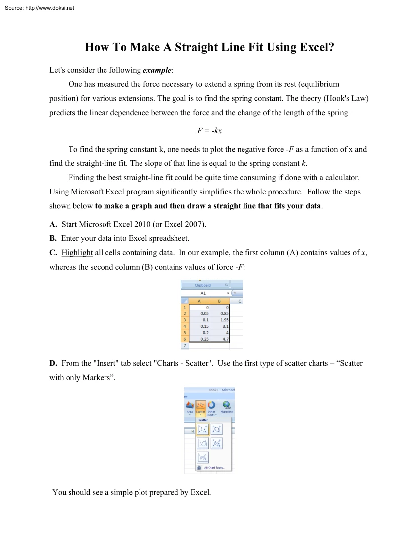
Source: http://www.doksinet How To Make A Straight Line Fit Using Excel? Lets consider the following example: One has measured the force necessary to extend a spring from its rest (equilibrium position) for various extensions. The goal is to find the spring constant The theory (Hooks Law) predicts the linear dependence between the force and the change of the length of the spring: F = -kx To find the spring constant k, one needs to plot the negative force -F as a function of x and find the straight-line fit. The slope of that line is equal to the spring constant k Finding the best straight-line fit could be quite time consuming if done with a calculator. Using Microsoft Excel program significantly simplifies the whole procedure. Follow the steps shown below to make a graph and then draw a straight line that fits your data. A. Start Microsoft Excel 2010 (or Excel 2007) B. Enter your data into Excel spreadsheet C. Highlight all cells containing data In our example, the first column (A)

contains values of x, whereas the second column (B) contains values of force -F: D. From the "Insert" tab select "Charts - Scatter" Use the first type of scatter charts – “Scatter with only Markers”. You should see a simple plot prepared by Excel. Source: http://www.doksinet E. Next step is to add axis labels and legend to the graph Select “Layout” tab from “Chart Tools”. Then add a header using the “Chart Title” button and add axis labels using “Axis Titles” button (both for horizontal and for vertical axes). Optionally, you may edit or simply remove the legend. Grab and drag a corner of the graph (chart) to enlarge its size F. The last step is to add the linear fit (a straight line fit) to your graph (chart) Click once anywhere inside the graph area. Select the “Layout” tab from “Chart Tools” Click on the “Trendline” icon and select the “Linear Trendline” option. You should see a graph similar to this: Now we can see the

straight line of the fit, but we do not know what the parameters of the equation are. To show the equation, click on “Trendline” and select “More Trendline Options” Then check the “Display Equation on chart” box. Source: http://www.doksinet The final result should look similar to the example shown below. From the equation for that straight line (y = 19.486x - 0002) we can conclude that the best estimate of the spring constant is: k = 19.49 (N/m), where 1949 (N/m) is the slope of the line and -0.002 (N) represents the y-intercept To change the number of decimal places in the trendline equation, right-click on the equation for the trendline and select option: "Format Trendline Label." Source: http://www.doksinet Next, select "Number" and increase or decrease the number of "Decimal places". MS Excel can be also used to fit more complicated equations (e.g, polynomial, exponential, logarithmic, etc.) using the same procedure, but with

different trendline options – “More Trendline Options”