Gépészet | Gépgyártástechnológia » Brakes and Clutches

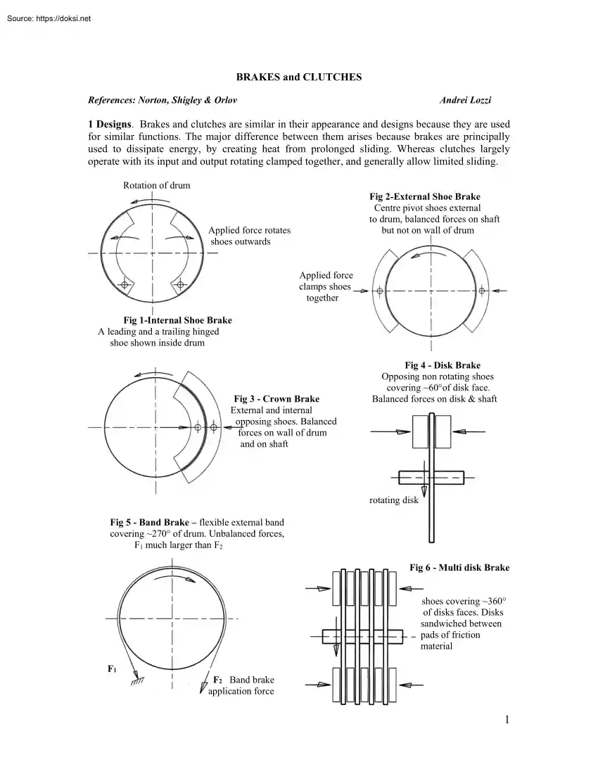
BRAKES and CLUTCHES References: Norton, Shigley & Orlov Andrei Lozzi 1 Designs. Brakes and clutches are similar in their appearance and designs because they are used for similar functions. The major difference between them arises because brakes are principally used to dissipate energy, by creating heat from prolonged sliding. Whereas clutches largely operate with its input and output rotating clamped together, and generally allow limited sliding. Rotation of drum Fig 2-External Shoe Brake Centre pivot shoes external to drum, balanced forces on shaft but not on wall of drum Applied force rotates shoes outwards Applied force clamps shoes together Fig 1-Internal Shoe Brake A leading and a trailing hinged shoe shown inside drum Fig 3 - Crown Brake External and internal opposing shoes. Balanced forces on wall of drum and on shaft Fig 4 - Disk Brake Opposing non rotating shoes covering ~60°of disk face. Balanced forces on disk & shaft rotating disk Fig 5 - Band Brake –

flexible external band covering ~270° of drum. Unbalanced forces, F1 much larger than F2 Fig 6 - Multi disk Brake shoes covering ~360° of disks faces. Disks sandwiched between pads of friction material F1 F2 Band brake application force 1 Fig 7 - Cone brake The drum and cone rotate and slide axially relative to each other. The force at the friction face is the applied force amplified by the inverse of sin of the cone angle. Rotating drum Sliding cone Applied force 2 Principle features of brakes: The usual analysis of brakes (we will drop any reference to clutches wherever practical) relies on one being able to make a number of unique simplifications: 1. Common friction material has a much lower compressive strength than what it usually makes contact with, ie steel or cast iron, by a factor of almost 100. We therefore assume that the friction pad is the only component that wears. 2. Due to the geometric properties of brake mechanisms the contact pressure on the friction face

is generally not uniform (eg shoe and band brakes). Nor in some case will the sliding velocity at the friction face be uniform (eg disk and cone brakes). 3. The maximum force that can be applied to a brake shoe will be reached when the maximum pressure ( pa ), somewhere on the brake shoe, is equal to the highest safe stress that can be applied to the friction material. Everywhere else p < pa 4. We will assume that the wear rate of the friction material is proportional to the product of δ ∝ Vp eq 1 the contact pressure and sliding velocity: The wear rate may be more complex than that, but the wear δ is always measured perpendicularly to the friction surface A preview of brake analysis Because the face of the pad in drum brakes cannot be kept parallel to the friction surface as they move, the wear will be not uniform. As a consequence that implies that the pressure, which causes the wear, will be equally not uniform. The force that can be applied to the shoe cannot be increased

beyond the point when the safe maximum compressive stress is reached somewhere on the face of the brake pad. It is then desirable to design brakes that have as uniform a pressure distribution as practical. In disk and cone brakes the relative sliding velocity cannot be the same over the whole face of the pad. Areas of the pad closer to the centre of rotation will have lower sliding velocities than areas further away. Consequently from eq1 we can expect non uniform pressure, non uniform wear or something in between. 2 In general the analysis of different styles of brakes begins with determining the wear distribution from the geometry of the mechanism that controls the movement. From eq1 the wear distribution reveals the pressure distribution. Integrating the pressure over the face of the pad gives us the forces and reactions. Integrating the product of the pressure and the coefficient of friction gives us the drag or torque that the brake generates. 3 A small leading shoe brake The

figure below shows a ‘small’ hinged brake shoe pushed into contact by the external force F onto a flat friction surface. Assuming that F is applied at the centre of pressure of the pad, a and b are the locations of the hinge centre, V is the sliding velocity, N is the resulting normal force between the surfaces and μN is the frictional or braking force. We can arrive at the forces acting on the shoe by taking moments about hinge centre O: b O µNa + Fb = Nb N ( µa − b) = − Fb  b  ∴ N = F    b − µa  eq 2 F a eq 3 V µN N Fig 8 A small flat hinged leading shoe brake Note that from eq 3 the externally applied force F is amplified by the factor: b/(µa-b). If µab this factor tends to infinity and for any initiating force F the brake will come on with increasing clamping force N, that is it will lock. The arrangement shown on Fig 8 is called a leading shoe brake, for obvious reasons. It is usually designed so that the amplifying factor is

moderate and such a brake is referred to as self-energising. This principle has been relied upon to provide braking for heavy or high performance machinery and may be seen as a passive mechanism that lead to modern power-assisted brakes. The fact that the proportions of a and b can be chosen such that the brake will self-lock is a feature of these brakes that can and is put to good use, but can also generate unexpected results should μ, the coefficient of friction, become suddenly large. The sort of embarrassing results that small boys experience, when they run about holding a stick in front of them, sliding the bottom end of the stick on ground. The above brake is referred to as ‘small’ because it can be assumed that the centre of pressure is very nearly also the centre of area. 3 4 Trailing shoe brake If in Fig 8 the direction of sliding V is reversed, the frictional force μN would also be reversed, and the this type of brake would will then be called a trailing shoe

brake. Taking moments about O would give different results from eq3 above: Fb = Nb + Nµa eq 4  ∴ N = F  b  µa + b  eq 5 Note that for any real values of a, b & μ the factor b/(µa+b) will always be less than 1. For a trailing shoe brake the clamping force will always be less than the externally applied force. Such brakes are safe in so far that we can be confident that they self-release, they cannot possibly lock. On the other hand they may require a great deal of force or power-assistance to generate a sufficient braking force. The internal shoe brake drum on Fig 1 has a trailing and a leading shoe. This is done for cheapness; typically a single hydraulic cylinder is used to push the two shoes apart at their top end. The leading shoe will do most of the braking and suffer most of the wear. In some installations 3 and 4 leading shoes have been used to provide powerful self-energising braking without expensive boosters. This was very effective for

sporting cars being driven around with gusto and alacrity, but risky when used on trucks, in so far that such trucks would have significantly reduced braking when travelling in reverse. Imagine the embarrassment backing down an incline to a big hole in the Fig 9 A 3 leading shoe drum brake ground, with a heavy load to be dumped, but being unable to stop using such a smashingly good brake as that shown on Fig 9. 5 Wear and pressure distributions As we said above, the mechanism determines the pads movement. If the pads are displaced unevenly, uneven wear will result and the wear distribution will be indicative of the pressure distribution. Figure 8 is redrawn below with a small rotation of the shoe imposed on it. You can show for yourself that the vertical displacement of the shoe, perpendicular to the friction face, increases with increasing θ, being the least directly below the pivot, at θ = 0, and a max at θa. eq 6 δ ∝ sin θ The pressure at the interface has to be proportional

to this wear ∴ p ∝ sin θ eq 7 The highest press pa take place at θa, therefore by ratio & proportions: sin θ eq 8 p = pa sin θ a Fig 10 4 Where pa has to be the maxim pressure at A that you can allow according to the material used. Consequently the pressure falls from A to B. The greater the angle covered by the shoe, ie θa- θ1, the greater will be the difference between the braking effect between points A and B. This is a property of all hinged shoes brakes, increasing the size of the shoe does not proportionally increase the braking effect. This suggests the use of multiple short shoes to make better use of the space available. For more predictable neutral performance accompanied by more uniform wear, centre pivot shoes are used. They may be inside or outside of a brake drum The crown brake shown on Fig 4 has centre pivot shoes opposite each other, on the inside and outside of a drum. The crown brake is a most compact design, it was expected to be used on small

vehicles with comparable wheels, Those cars have not as yet been adopted by the market, but maybe all we have to do is to wait. We will see later that the pads clamping force F can be very large, often considerably larger than the force due to gravity on the axles of a vehicle. Therefore to reduce the unbalanced forces on shafts, nearly always designers use opposing shoes, as on Fig1 & 2. To also reduce the stresses and therefore the mass of the drum or disk designs like the crown and disk brake are used. There are examples of what may appear to be the opposite of good design, but which turn out to have very useful applications. In a modern brake design for freight trains, single unbalanced external centre pivot shoes are used. Single shoes contacting the rim of the wheels reduce the number of parts, reducing the total costs, maintenance and hopefully breakdowns. These designs are heavier and generate less braking force but on the balance could be more cost effective. 6 External

centre pivot shoe brakes Figure 11 shows schematically an external centre pivot brake shoe. The displacement of the shoe face nearest the pin, that is the wear δ at θ=0, is e . At some angle θ the displacement perpendicular to the friction surface, in the same direction as the compressive stresses, is reduced to e cosθ . δ ∝ cosθ The pressure at the interface has to be proportional to this wear e p=p cosθ p ∝ cosθ Since the highest press must take place at at θ=0 and cos 0 = 1, by ratio & proportions: p = p 0 cosθ eq 9 δ=e cosθ θ Fig 11 pa e δ=e Fig11 and 12 presents the geometric details required to arrive at the major loads on a centre pivot external shoe brake. Fig 12 also serves as an example of the methods by which a brake design can be analysed The infinitesimal elements of the normal force and frictional force are: 5 dN eq 10 = pw · rdθ eq 10b µdN = µpw · rdθ where w is the brake pad’s width and r the radius of the drum. We will

separate these into X & Y components, integrate them over the arc of the symmetric shoe, allow for some necessary boundary conditions and finally arrive at the reaction forces RX & RY and brake torque. An additional and useful boundary condition that can be imposed is to locate the shoe pivot, at some particular x value, x = a, where the sum of the moments due to friction about a is 0. There the shoe will neither be a leading nor trailing shoe. From Fig 12 using d to be the perpendicular distance between the Infinitesimal frictional force µdN and the pivot at a. Setting the integral of the moment about a to 0 gives: θ1 M = 2 ∫ µ ⋅ dN ⋅ d = 0 , eq 11 d = a cosθ − r eq 11b a = 4r sin θ 1 (2θ 1 + sin 2θ 1 ) eq 12 01 giving: From symmetry we can state that the integrals of the Y component of the normal force dN and the integral of the X component of frictional force are zero, ie: θ1 ∫ dN ⋅ sin θ ⋅ dθ = 0 eq 13 −θ1 θ1 ∫θ µdN ⋅ sin θ

⋅ dθ = 0 − eq 14 Fig 12 1 The integral of the X component of the normal force dN will always point in the same direction, will not add to 0, and will give us the X component of the reaction at the pivot pin RX. θ1 p wr eq 15 R X = 2 ∫ dN ⋅ cosθ ⋅ dθ = 0 (2θ 1 + 2 sin θ 1 ) = − N 2 0 The integral of the Y component of dN gives us the Y component of the reaction RY: θ1 RY = 2 ∫ µdN ⋅ cosθ ⋅ dθ = 0 µp 0 wr (2θ 1 + 2 sin θ 1 ) = − µN 2 eq 16 The vertical reaction Ry multiplied by the arm length a gives us the torque generated by this brake Using also eqs 12 and 16 gives us the torque in terms of θ, µ, r and w : T = aµN = 2r 2 sin θµp o w eq 17 6 7 External hinged shoe brake Figure 13 shows an external leading shoe brake. Shoes internal to the drum can be described by similar variables to these, a major difference is that the normal force dN on the shoe would point inwards and X & Y its components change sign. To make overall

decisions on brake selection we will probably want to extract the application force F and the torque generated by this brake. To do this we equate the moments about the hinge pin at A to 0 These moments are due to the external force F and the pressure on the friction material: sin θ sin θ a c = (r-a cosθ), e = a sinθ eq 19a eq 19b M µ = ∫ µdNc eq 20 M N = ∫ dNe eq 21 eq 18 p = pa Fig13 The application force F must create a moment equal and opposite to the sum of these: F = MN + Mµ b And the torque must be equal to : T = ∫ µr ⋅ dN T = µp a wr 2 (cos θ 1 + cos θ 2 ) sin θ a eq 22 eq 23 eq 24 For a trailing shoe, the frictional force changes direction and sign. If your brake is made up of one of each of these shoes then the total application force and braking torque has to be the sum of the contribution of each shoe. 7 8 Band Brakes . Assuming a completely flexible band, as we did for belts in belt drives, we arrive at the tension in the band

increasing exponentially from the low tension side of the band, ie F2, to the high tension side F1. The torque generated by the brake is: T = ( F1 − F2 ) D 2 eq 25 In fig15 below the radial and tangential forces are balanced, on a section of the band rdθ wide: Fig 14 dF = μdN eq 26 dN = Fdθ eq 27 substituting dN out of eqs 26 & 27 and integrating for dF gives: F1 = F2 eμθ eq 28 We can also say that: dN=pwr dθ eq 29 which together with eq 27 gives: p = F/wr eq 30 Fig 15 eq 30 will give us the maximum and minimum pressure under the band at F1 and F2 , given the torque required from the brake eq 25, and the relationship between F1 and F2 by eq 28. The above tells us that the pressure under the band being proportional to the tension in the band varies exponentially from F2 to F1. Exponential functions being what they are this indicates that band brakes can have the highest variation in brake pad pressure of any brake, making them the most inefficient user of the

friction area. On the positive side band brakes can be made to generate very large torque for a relatively modest applied force F2, although they do require large surface areas, relatively large diameters and face widths. Notwithstanding their disadvantages band brakes can be made good use of where for example drums of large diameters has to be made to satisfy other requirements. 8 9 Disk brakes. Fig 16 shows schematically a new brake pad on the left of the disk and a worn-in pad on the right. The new pad when subjected to a force through its centre of area (CofA) generates uniform pressure over the face of the pad. This uniform pressure has a limited life expectancy. Because as the sliding velocity increases with radius so will the wear rate increase from the centre out. After a relatively short period of time a state of uniform wear will be established, where the pressure on the pads will decrease inversely with the radius, to maintain uniform wear over the face. pα 1/r eq 31

p = pa ri / r eq 32 Fig 16 The highest pressure will then take place at the inner radius ri 10 Uniform pressure. Assuming we have uniform pressure on the face of the brake pad, we can easily arrive at the total force on the face on the disk, under uniform pressure condition, F= ro ∫p a 2πr ⋅ dr = πp a (ro2 − ri 2 ) eq 33 ri given that the pressure has to be T = ro ∫p a ri µr 2πr ⋅ dr = 2 πp a µ (ro3 − ri3 ) 3 eq 34 the highest permissible pa. The integral is over annular bands dr high 2πr long, from the inner radius ri to the outer one ro. The torque (eq 34) generated by such a disk is just the integral of the pressure multiplied by the infinitesimal friction moment 12 Uniform wear For uniform wear we cannot use pa everywhere we, have to use the expression eq 32 for p to assure uniform wear. Torque is likewise ro F = ∫( ri ro T = ∫( ri p a ri )2πr ⋅ dr = 2πp a ri (ro − ri ) eq 35 r p a ri )µr 2πr ⋅ dr = πp a µri ( ro2 − ri

2 ) eq 36 r calculated using eq31 in equation eq 33, for the pressure. An interesting feature of disk brakes is that within a given outside diameter- 2ro the pressure at the max diameter will drop with decreasing inside diameter, (eq 31): po = pa ri/ro. To maximise torque for a given outer diameter, the inner diameter should be: ri = ro/√3. To show this you may find the max value of T with respect to ri Nevertheless this may not be the last word in disk brake proportions, possibly to dissipate heat, the front wheel of some motorcycles use disks of very large inner and outer diameters, which are clearly not to these proportions. Do you think you can detect the difference between new and bedded-in clutch plates, or disk brake pads in your vehicle? 9 12 Conical clutches at uniform wear. Cone clutches have many and tricky features but many an advantage. Seen on the right on fig 17, we may see that the front projection of a cone clutch is the same as a disk brake, but on the left

side we see that an annular band dr becomes dw = dr/sinα. The force F becomes N = F/sinα perpendicular to the friction face. To calculate for the axial for F, under condition of uniform wear we get the same value as for a plane disk: Fig 17 F = ro ∫( ri p a ri 2πr ⋅ dr ) sin α = 2πp a ri ( ro − ri ) sin α r eq 37 To integrate for torque the result is quite different because the effect of the larger normal force N comes into play: T = ro p a ri ∫ ( sin αr )µr 2πr ⋅ dr = ri µπp a ri ( ro2 − ri 2 ) 2 sin α eq 38 The denominator in eq 38 is an indication why cone brakes have a particular advantage. This amplifying effect can also be also a trap for the unwary. For small values of α a cone can become jammed into place requiring large forces to extract a non slipping cone. They have been used where a skilled operator would for example engage a cone brake and maintain the engagement as long as the torque remained high. As the torque fell off the operator

would progressively disengage the brake. Otherwise it would take special effort to extract the cone when the components came to a halt. 10 14 Heat dissipation from disk brake refs: R Limpert SAE and Shigley & Miscke ‘Standard Handbook of Machine Design’. Calculating, or more appropriately estimating, heat loss from a component to the environment is affected by many variables with messy interrelationships. These relationships are functions of air velocity, surface finish, surface optical properties and temperature differences, and apply to the component of interest as well as all other components that can have a thermal influence on that part. It is not surprising that ‘calculation’ of temperatures and heat flux is ‘fine tuned’ using experimental results. With more effective materials and improved oils the operating temperatures of brakes is continuously increasing. Heat can be lost from the friction surfaces by all the usual methods: conduction, convection and

radiation. For heavy slow moving machinery metal to metal conduction may be most significant. The thermal capacity of heavy components like brake drums can be used to modulate the temperature rises from large energy absorption, interspersed by periods of limited operation and low convective losses. Next, conduction and convection to air is most significant. Here the rate of loss is highly dependent with air velocity At high speed the air is turbulent and the heat transport coefficient may be 50 times larger than that at low velocity with laminar flow. A brake may operate very effectively at high speed but overheat, at low speeds cause such overheating that they blow out tires and boil the hydraulic fluid. Finally radiation plays a more significant part with increasing temperatures, being a function of the fourth power of absolute temperature. Radiation of heat is double edged, is so far as the brake components radiate to the surrounds but the surrounds radiates back to the brake, as

the surrounds gets hotter this heat loss mechanism becomes less effective. A method of estimation is as follows: Hdiss= hA(Tb-Te) Hdiss h A Tb Te heat dissipation rate J sec-1 total heat transfer coefficient area of brake brake temperature environment temperature h = hr+fvhc hr hc fv radiative transfer coefficient conductive transfer coefficient air velocity multiplying factor 11 Calculating the drop in the temperature of a disk during a cruise or stationary period. To begin to calculate the temperature drop in a disk that has been heated during a braking period to a temperature td above its environment’s temperature, we need to have an estimate of the total heat transfer rate from the disk to its environment. We can use either linear or non linear estimates for the heat transfer rate, that takes into account both radiative and convective effects. Linear estimates will underestimate the transfer rate at high and low temperatures but exaggerate at mid temperatures. Below we

have the heat transfer Htot as a quadratic function of temperature : Htot = (a1 ⋅ td 2 + a 2 ⋅ td + a3) + f (b1 ⋅ td 2 + b 2 ⋅ td + b3) The first term above represents the radiative component, the second the conductive one. Here f is a multiplicative factor that increases with air velocity, reflecting the greater heat transportation capacity of turbulent over laminar air flow. Note that this rate in the units of J/mm2 ∆C⁰ sec is a very small number as shown by the graph at bottom. For a disk of mass Mb specific heat cp and surface area of Ad, which has reached a temperature of td1 above ambient, subjected to a total heat transfer rate of Htot(td1) during a period of s seconds, we can first calculate the heat energy loss ∆E from the disk: Then we calculate the temp drop: Hence the new disk temperature: ∆E = Htot ⋅ Ad ⋅ td1 ⋅ s ∆temp = ∆E Mb ⋅ cp td 2 = td1 − ∆temp at time s Provided that the estimated new temperature td2 is well above ambient

temperature and the time interval s is a fraction of the total time available we can repeat the above calculation with Htot(Td2) for the next temperature at time 2s giving a smaller ∆E and a smaller ∆temp because: Htot(Td2) < Htot(td1) 10-6 Degrees C above ambient 12